Module 5.9 : Gradient Descent with Adaptive Learning Rate
Mitesh M. Khapra


AI4Bharat, Department of Computer Science and Engineering, IIT Madras
\sigma
1
x^1
x^2
x^3
x^4
y
y = f(x)=\frac{1}{1+e^{(-\mathbf{w^Tx}+b)}}
x=\{x^1,x^2,x^3,x^4\}
w=\{w^1,w^2,w^3,w^4\}
Given this network, it should be easy to see that given a single point (\(\mathbf{x},y\))
\nabla w^1= (f(\mathbf{x})-y)*f(\mathbf{x})*(1-f(\mathbf{x})*x^1
\nabla w^2= (f(\mathbf{x})-y)*f(\mathbf{x})*(1-f(\mathbf{x})*x^2 ..\text{so on}
If there are \(n\) points, we can just sum the gradients over all the \(n\) points to get the total gradient
What happens if the feature \(x^2\) is very sparse? (i.e., if its value is 0 for most inputs)
\(\nabla w^2\) will be 0 for most inputs (see formula) and hence \(w^2\) will not get enough updates
If \(x^2\) happens to be sparse as well as important we would want to take the updates to \(w^2\) more seriously.
Can we have a different learning rate for each parameter which takes care of the frequency of features?
Intuition
Decay the learning rate for parameters in proportion to their update history (more updates means more decay)
v_t=v_{t-1}+(\nabla w_t)^2
w_{t+1}=w_{t}-\frac{\eta}{\sqrt{v_t+\epsilon}}*\nabla w_{t}
... and a similar set of equations for \(b_t\)
Update Rule for AdaGrad
To see this in action we need to first create some data where one of the features is sparse
How would we do this in our toy network ?
Well, our network has just two parameters \(w \)and \(b\).
def do_adagrad(max_epochs):

  #Initialization
  w,b,eta = -2,-2,0.1
  v_w,v_b,eps = 0,0,1e-8
  for i in range(max_epochs):
    # zero grad
    dw,db = 0,0
    for x,y in zip(X,Y):

        #compute the gradients
        dw = grad_w(w,b,x,y)
        db = grad_b(w,b,x,y)

    #compute intermediate values
    v_w = v_w + dw**2
    v_b = v_b + db**2

    #update parameters
    w = w - eta*dw/(np.sqrt(v_w)+eps)
    b =b - eta*db/(np.sqrt(v_b)+eps)
Take some time to think about it
To see this in action we need to first create some data where one of the features is sparse
How would we do this in our toy network ?
Well, our network has just two parameters \(w \)and \(b\). Of these, the input/feature corresponding to \(b\) is always on (so can’t really make it sparse)
The only option is to make \(x\) sparse
Solution: We created 500 random \((x, y)\) pairs and then for roughly 80% of these pairs we set \(x\) to \(0\) thereby, making the feature for \(w\) sparse
def do_adagrad(max_epochs):

  #Initialization
  w,b,eta = -2,-2,0.1
  v_w,v_b,eps = 0,0,1e-8
  for i in range(max_epochs):
    # zero grad
    dw,db = 0,0
    for x,y in zip(X,Y):

        #compute the gradients
        dw += grad_w(w,b,x,y)
        db += grad_b(w,b,x,y)

    #compute intermediate values
    v_w = v_w + dw**2
    v_b = v_b + db**2

    #update parameters
    w = w - eta*dw/(np.sqrt(v_w)+eps)
    b =b - eta*db/(np.sqrt(v_b)+eps)
Take some time to think about it

There is something interesting that these 3 algorithms are doing for this dataset. Can you spot it?
Initially, all three algorithms are moving mainly along the vertical \((b)\) axis and there is very little movement along the horizontal \((w)\) axis
Why?
There is something interesting that these 3 algorithms are doing for this dataset. Can you spot it?
Initially, all three algorithms are moving mainly along the vertical \((b)\) axis and there is very little movement along the horizontal \((w)\) axis
Why? Because in our data, the feature corresponding to \(w\) is sparse and hence \(w\) undergoes very few updates
There is something interesting that these 3 algorithms are doing for this dataset. Can you spot it?
Initially, all three algorithms are moving mainly along the vertical \((b)\) axis and there is very little movement along the horizontal \((w)\) axis
Why? Because in our data, the feature corresponding to \(w\) is sparse and hence \(w\) undergoes very few updates ...on the other hand \(b\) is very dense and undergoes many updates
Such sparsity is very common in large neural networks containing \(1000s\) of input features and hence we need to address it
Let's see what AdaGrad does..
Adagrad
learning rate \(\eta_0\) = 0.1 for all the algorithms
Momentum \(\beta = 0.9\)
Number of points 500, 80% set to zero
Adagrad slows down near the minimum due to decaying learning rate
v_t=v_{t-1}+(\nabla w_t)^2
\nabla w=(f(x)-y) * f(x)*(1-f(x))*x
v_0=(\nabla w_0)^2
v_1=(\nabla w_0)^2+(\nabla w_1)^2
v_2=(\nabla w_0)^2+(\nabla w_1)^2+(\nabla w_2)^2
v_t=(\nabla w_0)^2+(\nabla w_1)^2+(\nabla w_2)^2+ \cdots+ (\nabla w_t)^2
Recall that,
Since \(x\) is sparse, the gradient is zero for most of the time steps.
Therefore, \(\dfrac{\eta}{\sqrt{v_t+\epsilon}}\) decays slowly.
Let's Examine it a bit more closely
v_t=v_{t-1}+(\nabla b_t)^2
\nabla b=(f(x)-y) * f(x)*(1-f(x))
v_0=(\nabla b_0)^2
v_1=(\nabla b_0)^2+(\nabla b_1)^2
v_2=(\nabla b_0)^2+(\nabla b_1)^2+(\nabla b_2)^2
v_t=(\nabla b_0)^2+(\nabla b_1)^2+(\nabla b_2)^2+ \cdots+ (\nabla b_t)^2
Recall that,
Though \(x\) is sparse, the gradient of \(b_t\) will not be zero for most of the time steps.(unless \(x\) takes a very large value)
Hence , \(\dfrac{\eta}{\sqrt{v_t+\epsilon}}\) decays rapidly.
Therefore, \(v_t\) grows rapidly.


\eta_t = \frac{\eta_0}{\sqrt{v_t+\epsilon}}
The effective learning rate
v_t = v_{t-1}+ (\nabla w_t)^2
\frac{\eta_0}{\sqrt{v_0+\epsilon}}
The effective learning rate decays gradually for the parameter \(w\).
\(v_t^w\) grows gradually
\frac{\eta_0}{\sqrt{v_0+\epsilon}} = \frac{0.1}{\sqrt{0.019}} = 0.72


\eta_t = \frac{\eta_0}{\sqrt{v_t+\epsilon}}
The effective learning rate
v_t = v_{t-1}+ (\nabla b_t)^2
\frac{\eta_0}{\sqrt{v_0+\epsilon}}
The effective learning rate decays rapidly for the parameter \(b\).
\(v_t^b\) grows rapidly because of accumulating gradients. For ex, \(\nabla b_0^2=-9.19^2=84.45\)
\frac{\eta_0}{\sqrt{v_0+\epsilon}} = \frac{0.1}{\sqrt{84.45}} = 0.01
Observe that in AdaGrad, \(v_t^w\) and \(v_t^b\) never become zero, despite the fact that the gradients become zero after some iterations.
v_t^b= v_{t-1}^b+ (\nabla b_t)^2
v_t^w = v_{t-1}^w+ (\nabla w_t)^2

By using a parameter specific learning rate it ensures that despite sparsity \(w\) gets a higher learning rate and hence larger updates
Further, it also ensures that if \(b\) undergoes a lot of updates its effective learning rate decreases because of the growing denominator
In practice, this does not work so well if we remove the square root from the denominator
By using a parameter specific learning rate it ensures that despite sparsity \(w\) gets a higher learning rate and hence larger updates
Further, it also ensures that if \(b\) undergoes a lot of updates its effective learning rate decreases because of the growing denominator
In practice, this does not work so well if we remove the square root from the denominator (something to ponder about)
What’s the flipside?
By using a parameter specific learning rate it ensures that despite sparsity \(w\) gets a higher learning rate and hence larger updates
Further, it also ensures that if \(b\) undergoes a lot of updates its effective learning rate decreases because of the growing denominator
In practice, this does not work so well if we remove the square root from the denominator (something to ponder about)
What’s the flipside? over time the effective learning rate for \(b\) will decay to an extent that there will be no further updates to \(b\)
Can we avoid this?
Intuition
Adagrad decays the learning rate very aggressively (as the denominator grows)
Update Rule for RMSprop
v_t = \beta v_{t-1}+(1-\beta)\nabla w_t^2
w_{t+1} = w_t - \frac{\eta}{\sqrt{v_t+\epsilon}}\nabla w_t
... and a similar set of equations for \(b_t\)
As a result, after a while, the frequent parameters will start receiving very small updates because of the decayed learning rate
To avoid this why not decay the denominator and prevent its rapid growth
v_t=v_{t-1}+\nabla b_t^2
\nabla b=(f(x)-y) * f(x)*(1-f(x))
v_0=\nabla b_0^2
v_1=\nabla b_0^2+\nabla b_1^2
v_2=\nabla b_0^2+\nabla b_1^2+\nabla b_2^2
v_t=\nabla b_0^2+\nabla b_1^2+\nabla b_2^2+ \cdots+ \nabla b_t^2
Recall that,
Therefore, \(\dfrac{\eta}{\sqrt{v_t+\epsilon}}\) decays rapidly for \(b\)
AdaGrad
v_t= \beta v_{t-1}+(1-\beta)(\nabla b_t)^2, \quad \beta\in[0,1)
v_0= 0.1\nabla b_0^2
v_1=0.09 \nabla b_0^2+0.1 \nabla b_1^2
\beta = 0.9
v_2=0.08 \nabla b_0^2+0.09 \nabla b_1^2+0.1 \nabla b_2^2
RMSProp
v_t= (1-\beta)\sum \limits_{\tau=0}^t \beta^{t-\tau} \nabla b_\tau^2
Therefore, \(\dfrac{\eta}{\sqrt{v_t+\epsilon}}\) decays slowly (compared to adagrad) for \(b\)
def do_rmsprop(max_epochs):
  #Initialization
  w,b,eta = -4,4,0.1
  beta = 0.5
  v_w,v_b,eps = 0,0,1e-4

  for i in range(max_epochs):
    # zero grad
    dw,db = 0,0

    for x,y in zip(X,Y):

        #compute the gradients
        dw = grad_w(w,b,x,y)
        db = grad_b(w,b,x,y)

    #compute intermediate values
    v_w = beta*v_w +(1-beta)*dw**2
    v_b = beta*v_b + (1-beta)*db**2

    #update parameters
    w = w - eta*dw/(np.sqrt(v_w)+eps)
    b =b - eta*db/(np.sqrt(v_b)+eps)
However, why there are oscillations?
Does it imply that after some iterations, there is a chance that the learning rate remains constant so that the algorithm possibly gets into an infinite oscillation around the minima?
RMSProp converged more quickly than AdaGrad by being less aggressive on decay
\eta = 0.1, \beta=0.5
Recall that in AdaGrad, \(v_t = v_{t-1}+\nabla w_t^2 \), never decreases despite the fact that the gradients become zero after some iterations. Is that the case for RMSProp?


Observe that the gradients \(d_{b}\) and\( d_w\) are oscillating after some iterations
RMSProp: \(v_t = \beta v_{t-1}+(1-\beta)(\nabla w_t^2)\)
AdaGrad: \(v_t = v_{t-1}+(\nabla w_t^2)\)
In the case of AdaGrad, the learning rate monotonically decreases due to the ever-growing denominator!
In the case of RMSProp, the learning rate may increase, decrease, or remains constant due to the moving average of gradients in the denominator.
The figure below shows the gradients across 500 iterations. Can you see the reason for the oscillation around the minimum?
What is the solution?
If learning rate is constant, there is chance that the descending algorithm oscillate around the local minimum.


\eta=0.05, \epsilon=0.0001
\eta=\frac{0.05}{\sqrt{10^{-4}}}
We have to set the initial learning rate appropriately, in this case, setting \(\eta=0.05\) solves this oscillation propblem.
What happens if we initialize the \(\eta_0\) with different values?
\eta_0=0.6
\eta_t=\frac{0.6}{\sqrt{v_t+\epsilon}}
v_t=\beta v_{t-1}+(1-\beta)(\nabla w_t)^2
\eta_0=0.1
\eta_t=\frac{0.1}{\sqrt{v_t+\epsilon}}
v_t=\beta v_{t-1}+(1-\beta)(\nabla w_t)^2
Which value for \(\eta_0\) is a good one ?
\eta_0=0.6
\eta_t=\frac{0.6}{\sqrt{v_t+\epsilon}}
v_t=\beta v_{t-1}+(1-\beta)(\nabla w_t)^2
\eta_0=0.1
\eta_t=\frac{0.1}{\sqrt{v_t+\epsilon}}
v_t=\beta v_{t-1}+(1-\beta)(\nabla w_t)^2
Which value for \(\eta_0\) is a good one ? Does this make any difference in terms of deciding how quickly the effective learning rate adapt to the gradient of the surface?
What happens if we initialize the \(\eta_0\) with different values?
Set \(\eta_0\) fixed to 0.6 in RMS prop (Top right)
It satisfies our wishlist: Decrease the learning rate at steep curvatures and increase the learning at gentle (or near flat) curvatures.
Let's set the value for \(\eta_0\) to 0.1 (bottom right)
Which one is better?
\text{in steep regions, say}, v_t = 1.25
\eta_t = \frac{0.6}{1.25} = 0.48
\eta_t = \frac{0.1}{1.25} = 0.08
\text{in flat regions, say}, v_t = 0.1
\eta_t = \frac{0.6}{0.1} = 6
\eta_t = \frac{0.1}{0.1} = 1
\(\eta_t = 0.08\) is better in a steep region and \(\eta_t=6\) is better in a gentle region. Therefore, we wish the numerator also to change wrt gradient/slope
Sensitive to initial learning rate, initial conditions of parameters and corresponding gradients (both RMSProp, AdaGrad)
If the initial gradients are large, the learning rates will be low for the remainder of training (in AdaGrad)
Later, if a gentle curvature is encountered, no way to increase the learning rate (In Adagrad)
AdaDelta
3. \rightarrow \Delta w_t = -\frac{\sqrt{u_{t-1}+\epsilon}}{\sqrt{v_t+\epsilon}} \nabla w_t
2. \rightarrow v_t = \beta v_{t-1}+(1-\beta)(\nabla w_t)^2
1. \rightarrow \nabla w_t
for \quad t \quad in \quad range(1,N):
Avoids setting initial learning rate \(\eta_0\).
Let's see how it does.
AdaDelta
3. \rightarrow \Delta w_t = -\frac{\sqrt{u_{t-1}+\epsilon}}{\sqrt{v_t+\epsilon}} \nabla w_t
5. \rightarrow u_t = \beta u_{t-1}+(1-\beta)(\Delta w_t)^2
4.\rightarrow w_{t+1}=w_t+\Delta w_t
2. \rightarrow v_t = \beta v_{t-1}+(1-\beta)(\nabla w_t)^2
1. \rightarrow \nabla w_t
for \quad t \quad in \quad range(1,N):
Avoids setting initial learning rate \(\eta_0\).
Since we use \(\Delta w_t\) to update the weights, it is called as Adaptive Delta
Let's see how it does.
Now the numerator, in the effective learning rate, is a function of past gradients (where as it was a constant in RMSprop, AdaGrad)
Observe that the \(u_t\) that we compute at \(t\) will be used only in the next iteration.
Also, notice that we take only a small fraction (\(1-\beta\)) of (\(\Delta w_t)^2\)
The question is, what difference does \(u_t\) make in adapting the learning rate?
v_t = \beta v_{t-1}+(1-\beta)\nabla w_t^2
v_t= \beta v_{t-1}+(1-\beta)(\nabla w_t)^2, \quad \beta\in[0,1)
v_0= 0.1\nabla w_0^2
v_1=0.09 \nabla w_0^2+0.1 \nabla w_1^2
\beta = 0.9
v_2=0.08 \nabla w_0^2+0.09 \nabla w_1^2+0.1 \nabla w_2^2
v_t= (1-\beta)\sum \limits_{\tau=0}^t \beta^{t-\tau} \nabla w_t^2

v_3=0.07 \nabla w_0^2+0.08 \nabla w_1^2+0.09 \nabla w_2^2+0.1 \nabla w_3^2
We want the learning rate to decrease
v_t = \beta v_{t-1}+(1-\beta)\nabla w_t^2
v_t= \beta v_{t-1}+(1-\beta)(\nabla w_t)^2, \quad \beta\in[0,1)
v_0= 0.1\nabla w_0^2
v_1=0.09 \nabla w_0^2+0.1 \nabla w_1^2
\beta = 0.9
v_2=0.08 \nabla w_0^2+0.09 \nabla w_1^2+0.1 \nabla w_2^2
v_t= (1-\beta)\sum \limits_{\tau=0}^t \beta^{t-\tau} \nabla w_t^2
v_3=0.07 \nabla w_0^2+0.08 \nabla w_1^2+0.09 \nabla w_2^2+0.1 \nabla w_3^2
We want the learning rate to increase
v_0= 0.1\nabla w_0^2
\Delta w_0 = -\frac{\sqrt{\epsilon}}{\sqrt{v_0+\epsilon}} \nabla w_0
u_0= 0.1 \Delta w_0^2
Starting at high curvature region
\(\Delta w_0 \ll \nabla w_0\) (if we ignore \(\epsilon\) in the den. Then \(\Delta w_0=-3.16\sqrt{\epsilon}\))
\(u_0 \ll v_0\) , because of squaring delta
w_{1}=w_0+\Delta w_0
A very small update (What we wish for)
\nabla w_0
\text{say,}\epsilon=10^{-6}
3. \rightarrow \Delta w_t = -\frac{\sqrt{u_{t-1}+\epsilon}}{\sqrt{v_t+\epsilon}} \nabla w_t
5. \rightarrow u_t = \beta u_{t-1}+(1-\beta)(\Delta w_t)^2
4.\rightarrow w_{t+1}=w_t+\Delta w_t
2. \rightarrow v_t = \beta v_{t-1}+(1-\beta)(\nabla w_t)^2
1. \rightarrow \nabla w_t
v_0= 0.1\nabla w_0^2
\Delta w_0 = -\frac{\sqrt{\epsilon}}{\sqrt{v_0+\epsilon}} \nabla w_0
u_0= 0.1 \Delta w_0^2
Starting at high curvature region
w_{1}=w_0+\Delta w_0
v_1= 0.08 \nabla w_0^2+0.1\nabla w_1^2
\Delta w_1 = -\frac{\sqrt{u_0+\epsilon}}{\sqrt{v_1+\epsilon}} \nabla w_1
u_1= 0.08 \Delta w_0^2+0.1 \Delta w_1^2
w_{2}=w_1+\Delta w_1
A smaller update.
\(u_0 \ll v_1\), therefore \(\Delta w_1 \ll \nabla w_1\)
If the gradient remains high, then the numerator grows more slowly than the denominator. Therefore, the rate of change of learning rate is determined by the previous gradients!
\nabla w_0
\nabla w_1
\(\Delta w_0 \ll \nabla w_0\) (if we ignore \(\epsilon\) in the den. Then \(\Delta w_0=-3.16\sqrt{\epsilon}\))
\(u_0 \ll v_0\) , because of squaring delta
A very small update (What we wish for)
\text{say,}\epsilon=10^{-6}
v_0= 0.1(\nabla w_0)^2
\Delta w_0 = -\frac{\sqrt{\epsilon}}{\sqrt{v_0+\epsilon}} \nabla w_0
u_0= 0.1 (\frac{\sqrt{\epsilon}}{\sqrt{v_0+\epsilon}} \nabla w_0)^2
Starting at high curvature region
w_{1}=w_0+\Delta w_0
\nabla w_0
\text{say,}\epsilon=10^{-6} \quad \beta=0.9
3. \rightarrow \Delta w_t = -\frac{\sqrt{u_{t-1}+\epsilon}}{\sqrt{v_t+\epsilon}} \nabla w_t
5. \rightarrow u_t = \beta u_{t-1}+(1-\beta)(\Delta w_t)^2
4.\rightarrow w_{t+1}=w_t+\Delta w_t
2. \rightarrow v_t = \beta v_{t-1}+(1-\beta)(\nabla w_t)^2
1. \rightarrow \nabla w_t
v_{-1}=0, \quad u_{-1}=0
t=0
Store A fraction of a history for next iteration
v_1= 0.9 v_0+ 0.1 (\nabla w_1)^2 = 0.09 (\nabla w_0)^2+0.1 (\nabla w_1)^2
\Delta w_1 = -\frac{\sqrt{u_0}}{\sqrt{v_1}} \nabla w_1
u_1= 0.09(\frac{\sqrt{\epsilon}}{\sqrt{v_0+\epsilon}} \nabla w_0)^2+0.1(\frac{\sqrt{u_0}}{\sqrt{v_1}} \nabla w_1)^2
w_{2}=w_1+\Delta w_1
t=1
v_2= 0.9 v_1+ 0.1 (\nabla w_2)^2 = 0.08 (\nabla w_0)^2+0.09 (\nabla w_1)^2+0.1(\nabla w_2)^2
\Delta w_2 = -\frac{\sqrt{u_1}}{\sqrt{v_2}} \nabla w_2
u_2= 0.08(\frac{\sqrt{\epsilon}}{\sqrt{v_0+\epsilon}} \nabla w_0)^2+0.09(\frac{\sqrt{u_0}}{\sqrt{v_1}} \nabla w_1)^2+0.1(\frac{\sqrt{u_1}}{\sqrt{v_2}} \nabla w_2)^2
w_{3}=w_2+\Delta w_2
t=2
ignoring \(\epsilon\)
\nabla w_1
\nabla w_2
v_0= 0.1(\nabla w_0)^2
u_0= 0.1 (\frac{\sqrt{\epsilon}}{\sqrt{v_0+\epsilon}} \nabla w_0)^2
Starting at high curvature region
\nabla w_0
\text{say,}\epsilon=10^{-6} \quad \beta=0.9
3. \rightarrow \Delta w_t = -\frac{\sqrt{u_{t-1}+\epsilon}}{\sqrt{v_t+\epsilon}} \nabla w_t
5. \rightarrow u_t = \beta u_{t-1}+(1-\beta)(\Delta w_t)^2
4.\rightarrow w_{t+1}=w_t+\Delta w_t
2. \rightarrow v_t = \beta v_{t-1}+(1-\beta)(\nabla w_t)^2
1. \rightarrow \nabla w_t
v_{-1}=0, \quad u_{-1}=0
t=0
v_1= 0.9 v_0+ 0.1 (\nabla w_1)^2 = 0.09 (\nabla w_0)^2+0.1 (\nabla w_1)^2
u_1= 0.09(\frac{\sqrt{\epsilon}}{\sqrt{v_0+\epsilon}} \nabla w_0)^2+0.1(\frac{\sqrt{u_0}}{\sqrt{v_1}} \nabla w_1)^2
t=1
v_2= 0.9 v_1+ 0.1 (\nabla w_2)^2 = 0.08 (\nabla w_0)^2+0.09 (\nabla w_1)^2+0.1(\nabla w_2)^2
u_2= 0.08(\frac{\sqrt{\epsilon}}{\sqrt{v_0+\epsilon}} \nabla w_0)^2+0.09(\frac{\sqrt{u_0}}{\sqrt{v_1}} \nabla w_1)^2+0.1(\frac{\sqrt{u_1}}{\sqrt{v_2}} \nabla w_2)^2
t=2
\nabla w_1
\nabla w_2
for each iteration:
Both \(v_t\) and \(u_t\) increase
However, the magnitude of \(u_t\) is less than the magnitude of \(v_t\) as we take only a fraction of the gradient squared.
Starting at high curvature region
\nabla w_0
\text{say,}\epsilon=10^{-6} \quad \beta=0.9
3. \rightarrow \Delta w_t = -\frac{\sqrt{u_{t-1}+\epsilon}}{\sqrt{v_t+\epsilon}} \nabla w_t
5. \rightarrow u_t = \beta u_{t-1}+(1-\beta)(\Delta w_t)^2
4.\rightarrow w_{t+1}=w_t+\Delta w_t
2. \rightarrow v_t = \beta v_{t-1}+(1-\beta)(\nabla w_t)^2
1. \rightarrow \nabla w_t
v_{-1}=0, \quad u_{-1}=0
\nabla w_1
\nabla w_2
for each iteration:
Both \(v_t\) and \(u_t\) increase
However, the magnitude of \(u_t\) is less than the magnitude of \(v_t\) as we take only a fraction of the gradient squared.
-\frac{\sqrt{u_{t-1}+\epsilon}}{\sqrt{v_t+\epsilon}} \nabla w_t
The effective learning rate in AdaDelta is given by
Therefore, at time step \(t\), the numerator in AdaDelta uses the accumulated history of gradients until the previous time step \((t-1)\).
-\frac{1}{\sqrt{v_t+\epsilon}} \nabla w_t
The effective learning rate in RMSprop is given by
Therefore, even in a surface with a steep curvature, it won't aggressively reduce the learning rate like RMSProp.
In low curvature region
\nabla w_i
v_i= 0.034 \nabla w_0^2+0.038 \nabla w_1^2+ \cdots +0.08 \nabla w_{i-1}^2+0.1\nabla w_i^2
\Delta w_i = -\frac{\sqrt{u_{i-1}+\epsilon}}{\sqrt{v_i+\epsilon}} \nabla w_1
u_i= 0.034 \Delta w_0^2+0.038 \Delta w_1^2+\cdots+0.08\Delta w_{i-1}^2+0.1\Delta w_i^2
w_{i+1}=w_i+\Delta w_i
After some \(i\) iterations, the \(v_t\) will start decreasing and the ratio of the numerator to the denominator starts increasing.
If the gradient remains low for a subsequent time steps, then the learning rate grows accordingly.
Therefore, AdaDelta allows the numerator to increase or to decrease based on the current and past gradients.
\text{say,}\epsilon=10^{-6} \quad \beta=0.9
3. \rightarrow \Delta w_t = -\frac{\sqrt{u_{t-1}+\epsilon}}{\sqrt{v_t+\epsilon}} \nabla w_t
5. \rightarrow u_t = \beta u_{t-1}+(1-\beta)(\Delta w_t)^2
4.\rightarrow w_{t+1}=w_t+\Delta w_t
2. \rightarrow v_t = \beta v_{t-1}+(1-\beta)(\nabla w_t)^2
1. \rightarrow \nabla w_t
v_{-1}=0, \quad u_{-1}=0
def do_adadelta(max_epochs):
  #Initialization
  w,b= -4,-4
  beta = 0.99
  v_w,v_b,eps = 0,0,1e-4
  u_w,u_b = 0,0

  for i in range(max_epochs):
    dw,db = 0,0
    for x,y in zip(X,Y):

        #compute the gradients
        dw += grad_w(w,b,x,y)
        db += grad_b(w,b,x,y)

    v_w = beta*v_w + (1-beta)*dw**2
    v_b = beta*v_b + (1-beta)*db**2

    delta_w = dw*np.sqrt(u_w+eps)/(np.sqrt(v_w+eps))
    delta_b = db*np.sqrt(u_b+eps)/(np.sqrt(v_b+eps))
    u_w = beta*u_w + (1-beta)*delta_w**2
    u_b = beta*u_b + (1-beta)*delta_b**2


    w = w - delta_w
    b = b - delta_b

It starts off with a (moderately) high curvature region and after 35 iterations it reaches the minimum


v_t = 0.9 v_{t-1}+0.1(\nabla w_t)^2
u_t = 0.9 u_{t-1}+0.1(\frac{\sqrt{u_{t-1}}}{\sqrt{v_t}}\nabla w_t)^2
Note the shape and magnitude of both \(v_t\) and \(u_t\).
The shape is alike but the magnitude differs
Implies that if \(v_t\) grows, \(u_t \) will also grow proportionally and vice a versa
AdaDelta
AdaDelta
\dfrac{\sqrt{u_w+\epsilon}}{\sqrt{v_w+\epsilon}}
\dfrac{0.013}{\sqrt{v_t^w+\epsilon}}


AdaDelta
RMSProp
AdaDelta
AdaDelta
Let's initialize the RMSProp with \(\eta_0=0.013\) (Assume, we do it by chance) and AdaDelta at \(w_0=-4,b_0=-4\)
AdaDelta Converged more quickly than RMSprob as its learning rate is wisely adapted.
RMSProp decays the learning rate aaggressively than AdaDelta as we can see from the plot on the left.
Which algorithm converges quickly?Guess

Let's put all these together in one place
Adam (Adaptive Moments)
Intuition
Do everything that RMSProp and AdaDelta does to solve the decay problem of Adagrad
m_t = \beta_1m_{t-1}+(1-\beta_1)\nabla w_t
\hat{m_t} =\frac{m_t}{1-\beta_1^t}
v_t = \beta_2 v_{t-1}+(1-\beta_2)(\nabla w_t)^2
w_{t+1}=w_t-\frac{ \eta}{\sqrt{\hat{v_t}}+\epsilon}\hat{m_t}
\hat{v_t} =\frac{v_t}{1-\beta_2^t}
Incorporating classical
momentum
\(L^2\) norm
Plus use a cumulative history of the gradients
Typically, \(\beta_1=0.9\), \(\beta_2=0.999\)
def do_adam_sgd(max_epochs):

  #Initialization
  w,b,eta = -4,-4,0.1
  beta1,beta2 = 0.9,0.999
  m_w,m_b,v_w,v_b = 0,0,0,0

  for i in range(max_epochs):
    dw,db = 0,0
    eps = 1e-10
    for x,y in zip(X,Y):

        #compute the gradients
        dw = grad_w_sgd(w,b,x,y)
        db = grad_b_sgd(w,b,x,y)

    #compute intermediate values
    m_w = beta1*m_w+(1-beta1)*dw
    m_b = beta1*m_b+(1-beta1)*db
    v_w = beta2*v_w+(1-beta2)*dw**2
    v_b = beta2*v_b+(1-beta2)*db**2

    m_w_hat = m_w/(1-np.power(beta1,i+1))
    m_b_hat = m_b/(1-np.power(beta1,i+1))
    v_w_hat = v_w/(1-np.power(beta2,i+1))
    v_b_hat = v_b/(1-np.power(beta2,i+1))

    #update parameters
    w = w - eta*m_w_hat/(np.sqrt(v_w_hat)+eps)
    b = b - eta*m_b_hat/(np.sqrt(v_b_hat)+eps)
Million Dollar Question: Which algorithm to use?
Adam seems to be more or less the default choice now \((\beta_1 = 0.9, \beta_2 = 0.999 \ \text{and} \ \epsilon = 1e^{-8} )\).
Although it is supposed to be robust to initial learning rates, we have observed that for sequence generation problems \(\eta = 0.001, 0.0001\) works best
Having said that, many papers report that SGD with momentum (Nesterov or classical) with a simple annealing learning rate schedule also works well in practice (typically, starting with \(\eta = 0.001, 0.0001 \)for sequence generation problems)
Adam might just be the best choice overall!!
Some works suggest that there is a problem with Adam and it will not converge in some cases. Also, it is observed that the models trained using Adam optimizer usually don't generalize well.
Explanation for why we need bias correction in Adam
Update Rule for Adam
m_t = \beta_1m_{t-1}+(1-\beta_1)\nabla w_t
\hat{m_t} =\frac{m_t}{1-\beta_1^t}
v_t = \beta_2 v_{t-1}+(1-\beta_2)(\nabla w_t)^2
w_{t+1}=w_t-\frac{ \eta}{\sqrt{\hat{v_t}}+\epsilon}\hat{m_t}
\hat{v_t} =\frac{v_t}{1-\beta_2^t}
Note that we are taking a running average of the gradients as \(m_t\)
The reason we are doing this is that we don’t want to rely too much on the current gradient and instead rely on the overall behaviour of the gradients over many timesteps
One way of looking at this is that we are interested in the expected value of the gradients and not on a single point estimate computed at time t
However, instead of computing \(E[\nabla w_t]\) we are computing \(m_t\) as the exponentially moving average
Ideally we would want \(E[m_t ]\) to be equal to \(E[\nabla w_t ]\)
Let us see if that is the case
Recall the momentum equations from module 5.4
u_t = \beta u_{t-1}+ \nabla w_t
u_t = \sum \limits_{\tau=1}^t \beta^{t-\tau} \nabla w_{\tau}
What we have now in Adam is a slight modification to the above equation (let's treat \(\beta_1\) as \(\beta\) )
m_t = \beta m_{t-1}+(1-\beta)\nabla w_t
\rbrace
m_t = (1-\beta)\sum \limits_{\tau=1}^t \beta^{t-\tau} \nabla w_{\tau}
m_0 = 0
m_1 = \beta m_0+(1-\beta)\nabla w_1=(1-\beta)\nabla w_1
m_2 =\beta m_1 + (1-\beta) \nabla w_2
=\beta (1-\beta) \nabla w_1+ (1-\beta) \nabla w_2
= (1-\beta) (\beta\nabla w_1+ \nabla w_2)
m_3=\beta m_2 + (1-\beta) \nabla w_3
=\beta ((1-\beta) (\beta\nabla w_1+ \nabla w_2) )+(1-\beta) \nabla w_3
=(1-\beta) (\beta^2 \nabla w_1+\beta \nabla w_2)+(1-\beta) \nabla w_3
m_3 = (1-\beta)\sum \limits_{\tau=1}^3 \beta^{t-\tau} \nabla w_{\tau}
Recall the momentum equations from module 5.4
u_t = \beta u_{t-1}+ \nabla w_t
u_t = \sum \limits_{\tau=0}^t \beta^{t-\tau} \nabla w_{\tau}
What we have now in Adam is a slight modification to the above equation
m_t = \beta m_{t-1}+(1-\beta)\nabla w_t
\rbrace
m_t = (1-\beta)\sum \limits_{\tau=1}^t \beta^{t-\tau} \nabla w_{\tau}
Let's take expectation on both sides
E[m_t] =E[ (1-\beta)\sum \limits_{\tau=1}^t \beta^{t-\tau} \nabla w_{\tau}]
E[m_t] = (1-\beta)\sum \limits_{\tau=1}^t E[ \beta^{t-\tau} \nabla w_{\tau}]
E[m_t] = (1-\beta)\sum \limits_{\tau=1}^t \beta^{t-\tau} E[ \nabla w_{\tau}]
Assumption: All \(\nabla w_\tau\) comes from the same distribution,i.e.,
\(E[\nabla w_\tau] = E[\nabla w] \quad \forall \tau\)
E[m_t] = E[ \nabla w](1-\beta)
\sum \limits_{\tau=1}^t \beta^{t-\tau}
E[m_t] = E[ \nabla w](1-\beta)
(\beta^{t-1}+\beta^{t-2}+\cdots+\beta^{0})
E[m_t] = E[ \nabla w](1-\beta)
\frac{1-\beta^{t}}{1-\beta}
E[m_t] = E[ \nabla w](1-\beta^{t})
The last ratio is the sum of GP with common ratio \(\beta\)
E[\frac{m_t}{1-\beta^{t}}] = E[ \nabla w]
E[\hat{m_t}] = E[ \nabla w] \quad \text{where,} \hat{m_t}=\frac{m_t}{1-\beta^{t}}
Hence we apply the bias correction because then the expected value of \(\hat{m_t}\) is the same as the expected value of \(E[\nabla w_t]\)
Let's take expectation on both sides

Assume that we have only noisy observations
Estimate the true function using
Exponentially weighted (without bias correction)
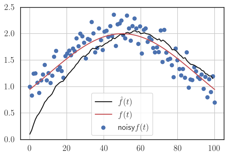
As expected, it gives a poor approximation for the first few iterations (obvious from the plot, it is biased towards zero)
Let's see the bias-corrected version of it
Bias correction is the problem of exponential averaging: Illustrative example
Assume that we have only noisy observations
Estimate the true function using
Exponentially weighted (with bias correction)

Bias correction is the problem of exponential averaging: Illustrative example
What if we don't do bias correction?
"..a lack of initialization bias correction would lead to initial steps that are much larger" [from the paper]
v_t=\beta_2 v_{t-1}+ (1-\beta_2)(\nabla w_t)^2, \quad \beta_2=0.999
Suppose, \(\nabla w_0=0.1\)
v_0=0.999 * 0+ 0.001(0.1)^2 = 0.00001
\eta_t=\frac{1}{\sqrt{0.00001}}=316.22
v_2=0.999 * v_0+ 0.001(0)^2 = 0.0000099
\eta_t=\frac{1}{\sqrt{0.0000099}}=316.38
Suppose, \(\nabla w_0=0.1\)
v_0=0.999 * 0+ 0.001(0.1)^2 = 0.00001
\hat{v}_0=\frac{v_0}{1-0.999} = \frac{0.00001}{0.001} = 0.01
\eta_t=\frac{1}{\sqrt{0.01}}=10
v_2=0.999 * v_0+ 0.001(0)^2 = 0.0000099
\eta_t=\frac{1}{\sqrt{0.0052}}=13.8
\hat{v}_0=\frac{v_0}{1-0.999^2} = \frac{0.0000099}{0.0019} = 0.0052
Therefore, doing a bias correction attenuates the initial learning to a greater extent.
What if we don't do bias correction?
Adam
Adam-No-BC
"..a lack of initialization bias correction would lead to initial steps that are much larger" [from the paper]


\eta_t=\frac{ \eta_0}{\sqrt{v_t}+\epsilon}
\eta_t=\frac{ \eta_0}{\sqrt{\hat{v_t}}+\epsilon}
\beta_2=0.999, \quad \eta_0=0.1
Is doing a bias correction a must?
No. For example, the Keras framework doen't implement bias correction

Let's revisit \(L^p\) norm
L^p=(|x_1|^p+|x_2|^p+\cdots+|x_n|^p)^{\frac{1}{p}}
In order to visualize it, let's fix \(L^p=1\) and vary \(p\)
1=(|x_1|^p+|x_2|^p)^{\frac{1}{p}}
1^p=|x_1|^p+|x_2|^p
1=|x_1|^p+|x_2|^p
We can choose any value for \(p \ge 1\)
However, you might notice, if \(p \rightarrow \infty\), it can simply be replaced with \(max(x_1,x_2,\cdots,x_n)\)
\(|x|\), raised to a high value of \(p\), becomes too small to represent. This leads to numerical instability in calculations.
So, what is the point we are trying to make?
Therefore, we can replace the \(\sqrt{v_t}\) by the \(\max()\) norm as follows
v_t=\max(\beta_2^{t-1}|\nabla w_1|,\beta_2^{t-2}|\nabla w_2|,\cdots,|\nabla w_t|)
v_t=\max(\beta_2v_{t-1},|\nabla w_t|)
w_{t+1}=w_t-\frac{\eta_0}{v_t}\nabla \hat{m}_t
Observe that we didn't use bias corrected \(v_t\) as max norm is not susceptible to initial zero bias.
v_t = \beta_2 v_{t-1}+(1-\beta_2)(\nabla w_t)^2
w_{t+1}=w_t-\frac{ \eta}{\sqrt{\hat{v_t}}+\epsilon}\hat{m_t}
\hat{v_t} =\frac{v_t}{1-\beta_2^t}
Recall, the equation of \(v_t\) from Adam
We call \(\sqrt{v_t}\) as \(L^2\) norm. Why not replace it with \(\max() (L^{\infty}) \) norm?
Let's see an illustrative example for this.
Assume that we have only noisy observations
Estimate the true function using
max norm, \(max(\beta v_{t-1},|\text{noisy} f(t)|)\)
Max norm is not susceptible to bias towards zero (i.e., zero initialization)

So, what is the point we are trying to make?
(v_t)^{\frac{1}{p}} = (\beta_2 v_{t-1}+(1-\beta_2)(\nabla w_t)^2)^{\frac{1}{p}}
We used \(L^2\) norm, \(\sqrt{v_t}\), in Adam. Why don't we just generalize it to \(L^p\) norm?
As discussed, for larger values of \(p\) ,\(L^p\) norm becomes numerically unstable.
However, as \(p \rightarrow \infty\) it becomes stable and can be repleaced with \(max()\) function.
v_t = \beta_2^p v_{t-1}+(1-\beta_2^p)|\nabla w_t|^p
Let's define
(v_t)^{\frac{1}{p}} = (\beta_2^p v_{t-1}+(1-\beta_2^p)|\nabla w_t|^p)^{\frac{1}{p}}
\lim\limits_{p \to \infty}(v_t)^{\frac{1}{p}} =\lim\limits_{p \to \infty}\Big((1-\beta_2^p) \sum \limits_{\tau=1}^t \beta_2^{(t-\tau)p} |\nabla w_t|^p\Big)^{\frac{1}{p}}
=\lim\limits_{p \to \infty}(1-\beta_2^p)^{\frac{1}{p}} \lim\limits_{p \to \infty} \Big(\sum \limits_{\tau=1}^t \big(\beta_2^{(t-\tau)} |\nabla w_t|\big)^p\Big)^{\frac{1}{p}}
=\lim\limits_{p \to \infty} \Big(\sum \limits_{\tau=1}^t \big(\beta_2^{(t-\tau)} |\nabla w_t|\big)^p\Big)^{\frac{1}{p}}
=\max(\beta_2^{t-1}|\nabla w_1|,\beta_2^{t-2}|\nabla w_2|,\cdots,|\nabla w_t|)
v_t=\max(\beta_2 v_{t-1},|\nabla w_t|), \quad \beta_2=0.999
Suppose that we initialize \(w_0\) such that the gradient at the \(w_0\) is high
Suppose further that the gradients for the next subsequent iterations are also zero (because \(x\) is sparse.)

\nabla w_t
Ideally, we don't want the learning rate to change (especially, increase) its value when \(\nabla w_t=0\) (because \(x=0\))
v_t=\max(\beta_2 v_{t-1},|\nabla w_t|), \quad \beta_2=0.999
v_0=\max(0,|\nabla w_0|)=1
v_1=\max(0.999*1,0|)=0.999
Ideally, we don't want the learning rate to change (especially, increase) its value when \(\nabla w_t=0\) because \(x=0\)
\eta_t=\frac{1}{1}=1
\eta_t=\frac{1}{0.999}=1.001
v_2=\max(0.999,1)=1


\eta_t=\frac{1}{1}=1
50% of input is zero
The problem with exponential averaging (even with bias correction) is that it increases the learning rate despite \(\nabla w_t=0\)
v_t=\beta_2 v_{t-1}+ (1-\beta_2)(\nabla w_t)^2, \quad \beta_2=0.999
v_0=0.999 * 0+ 0.001(\nabla w_0)^2 = 0.001
v_1=0.999*(0.001)+ 0.001(0)^2 = 0.000999
\eta_t=\frac{1}{\sqrt{1}}=1
\eta_t=\frac{1}{\sqrt{0.499}}=1.41
\hat{v_0}=\frac{0.001}{1-0.999}=1
\hat{v_1}=\frac{0.000999}{1-0.999^2}=0.499

Let's see the behaviour of exponential averaging and Max norm for the following gradient profile


Exponential averaging in RMSprop keeps increasing the learning rate where as Max norm is quite conservative in increasing the learning rate
\frac{1}{\max(0,1.16)}=0.86
\frac{1}{v_0}=\frac{1}{1.34}=0.74
For the first few iterations ,\(t=(0,1,\cdots,10)\), the gradient is high and then it gradually decreases.
In terms of convergence, both the algorithms converge to the minimum eventually as the loss surface is smooth and convex
In general, having low learning rate at steep surfaces and high learning rate at gentle surfaces is desired.
For a smooth convex loss surface, exponential averaging wins as increasing the learning rate is not a harm.
MaxProp
v_t = max(\beta v_{t-1},|\nabla w_t|)
Update Rule for RMSProp
v_t = \beta v_{t-1}+(1-\beta)(\nabla w_t)^2
w_{t+1}=w_t-\frac{ \eta}{\sqrt{v_t}+\epsilon}\nabla w_t
Update Rule for MaxProp
w_{t+1}=w_t-\frac{ \eta}{v_t+\epsilon}\nabla w_t
We can extend the same idea to Adam and call it AdaMax
In fact, using max norm in place of \(L^2\) norm was proposed in the same paper where Adam was proposed.
AdaMax
v_t = max(\beta_2v_{t-1},|\nabla w_t|)
w_{t+1}=w_t-\eta \frac{ \hat{m_t}}{v_t+\epsilon}
Update Rule for Adam
m_t = \beta_1m_{t-1}+(1-\beta_1)\nabla w_t
\hat{m_t} =\frac{m_t}{1-\beta_1^t}
v_t = \beta_2 v_{t-1}+(1-\beta_2)(\nabla w_t)^2
w_{t+1}=w_t-\frac{ \eta}{\sqrt{\hat{v_t}}+\epsilon}\hat{m_t}
\hat{v_t} =\frac{v_t}{1-\beta_2^t}
Update Rule for AdaMax
m_t = \beta_1m_{t-1}+(1-\beta_1)\nabla w_t
\hat{m_t} =\frac{m_t}{1-\beta_1^t}
w_{t+1}=w_t-\frac{ \eta}{v_t+\epsilon}\hat{m_t}
Note that bias correction for \(v_t\) is not required for Max function, as it is not susceptible to initial bias towards zero.
50% of the elements in input \(x\) is set to zero randomly. The weights are updated using SGD with \(\beta_2=0.999, \eta_0=0.025\)
Observe that the weights (\(w\)) get updated even when \(x=0 (\implies \nabla w_t=0)\), that is because of momentum not because of the current gradient.

At 10th iteration

dw
Both Adam and Adamax have moved in the same direction. Let's look at the gradients
v_0 =\frac{ 0.001*(-0.0314)^2}{0.001}=0.00098
\eta_t = \frac{0.025}{\sqrt{0.00098}}=0.79
v_0=\max(0,|-0.0314|)=0.0314
\eta_t = \frac{0.025}{0.0314}=0.79

Adam
Adamax

Adamax Works good for SGD
For Batch-Gradient Descent
Adam Wins the race
def do_adamax_gd(max_epochs):

  #Initialization
  w,b,eta = -4,-4,0.1
  beta1,beta2 = 0.9,0.99
  m_w,m_b,v_w,v_b = 0,0,0,0
  m_w_hat,m_b_hat,v_w_hat,v_b_hat = 0,0,0,0


  for i in range(max_epochs):
    dw,db = 0,0
    eps = 1e-10

    for x,y in zip(X,Y):

        #compute the gradients
        dw += grad_w_sgd(w,b,x,y)
        db += grad_b_sgd(w,b,x,y)


    #compute intermediate values
    m_w = beta1*m_w+(1-beta1)*dw
    m_b = beta1*m_b+(1-beta1)*db
    v_w = np.max([beta2*v_w,np.abs(dw)])
    v_b = np.max([beta2*v_b,np.abs(db)])

    m_w_hat = m_w/(1-np.power(beta1,i+1))
    m_b_hat = m_b/(1-np.power(beta1,i+1))

    #update parameters
    w = w - eta*m_w_hat/(v_w+eps)
    b = b - eta*m_b_hat/(v_b+eps)
def do_adamax_sgd(max_epochs):

  #Initialization
  w,b,eta = -4,-4,0.1
  beta1,beta2 = 0.9,0.99
  m_w,m_b,v_w,v_b = 0,0,0,0
  m_w_hat,m_b_hat,v_w_hat,v_b_hat = 0,0,0,0


  for i in range(max_epochs):
    dw,db = 0,0
    eps = 1e-10

    for x,y in zip(X,Y):

        #compute the gradients
        dw += grad_w_sgd(w,b,x,y)
        db += grad_b_sgd(w,b,x,y)


    #compute intermediate values
    m_w = beta1*m_w+(1-beta1)*dw
    m_b = beta1*m_b+(1-beta1)*db
    v_w = np.max([beta2*v_w,np.abs(dw)])
    v_b = np.max([beta2*v_b,np.abs(db)])

    m_w_hat = m_w/(1-np.power(beta1,i+1))
    m_b_hat = m_b/(1-np.power(beta1,i+1))

    #update parameters
    w = w - eta*m_w_hat/(v_w+eps)
    b = b - eta*m_b_hat/(v_b+eps)
Intuition
We know that NAG is better than Momentum based GD
We just need to modify \(m_t\) to get NAG
Why not just incorporate it with ADAM?
Update Rule for Adam
m_t = \beta_1 m_{t-1}+(1-\beta_1)\nabla w_t
\hat{m_t} =\frac{m_t}{1-\beta_1^t}
v_t = \beta_2 v_{t-1}+(1-\beta_2)(\nabla w_t)^2
w_{t+1}=w_t-\frac{ \eta}{\sqrt{\hat{v_t}}+\epsilon}\hat{m_t}
\hat{v_t} =\frac{v_t}{1-\beta_2^t}
Recall the equation for Momentum
u_t=\beta u_{t-1}+ \nabla w_{t}
Recall the equation for NAG
w_{t+1}=w_t - \eta u_t
u_t = \beta u_{t-1}+ \nabla (w_t - \beta \eta u_{t-1})
w_{t+1} = w_t - \eta u_t
We skip the multiplication of factor \(1-\beta\) with \(\nabla w_t\) for brevity
g_t = \nabla (w_t - \eta \beta m_{t-1})
m_t = \beta m_{t-1}+ g_t
w_{t+1} = w_t - \eta m_t
NAG
Observe that the momentum vector \(m_{t-1}\) is used twice (while computing gradient and current momentum vector). As a consequence, there are two weight updates (which is costly for big networks)!
\lbrace
Look ahead

w_0
\nabla w_0
w_1 = w_0 -\nabla(w_0-0)
w_1
g_1 = \nabla (w_1-\beta m_0))
g_0=\nabla w_0
\eta = 1
m_0=g_0
m_{-1} = 0
w_1-\beta m_0
\nabla (w_1-\beta \nabla w_0)
m_1=\beta m_0 +g_1

w_2 = w_1 -m_1 = w_1-(\beta m_0 +\nabla(w_1-\beta m_0))
g_t = \nabla (w_t - \beta m_{t-1})
m_t = \beta m_{t-1}+ g_t
w_{t+1} = w_t - \eta m_t
NAG
Observe that the momentum vector \(m_{t-1}\) is used twice (while computing gradient and current momentum vector). As a consequence, there are two weight updates (which is costly for big networks)!
\lbrace
Look ahead
w_0
\nabla w_0
w_1 = w_0 -\nabla(w_0-0)
w_1
g_1 = \nabla (w_1-\beta m_0)
g_0=\nabla w_0
\eta = 1
m_0=g_0
m_{-1} = 0
w_2
m_1=\beta m_0 +g_1
w_2 = w_1 -m_1 = w_1-(\beta m_0 +\nabla(w_1-\beta m_0))
Is there a way to fix this?
w_0
\nabla w_0
w_1 = w_0 -\nabla(w_0-0)
w_1
g_1 = \nabla (w_1-\beta m_0)
g_0=\nabla w_0
\eta = 1
m_0=g_0
m_{-1} = 0
w_2
m_1=\beta m_0 +g_1
w_2 = w_1 -m_1 = w_1-(\beta m_0 +\nabla(w_1-\beta m_0))
w_1 = w_0 -\nabla(w_0-0)
g_1 = \nabla (w_1-\beta m_0)
Why don't we do this look ahead in the previous time step? Because \(\beta m_0 \) is from the previous time step only!)
w_1 - \beta m_0 = (w_0 -\nabla(w_0-0))-\beta m_0
g_{t+1} = \nabla w_{t}
m_{t+1} = \beta m_{t}+ g_{t+1}
w_{t+1} = w_t - \eta ( \beta m_{t+1}+g_{t+1})
Rewritten NAG
\eta = 1
m_{0} = 0
g_1=\nabla w_0
w_0
\nabla w_0
m_1 = \beta m_0+g_1 = g_1
w_1 = w_0-\beta g_1-g_1
w_1
g_2=\nabla w_1
\nabla w_1
m_2 = \beta m_1+g_2=\beta g_1+g_2
w_2 = w_1- (\beta(\beta g_1+g_2)+g_2)
Now, look ahead is computed only at the momentum step \(m_{t+1}\)
w_0-\beta g_1
However, the gradient of look ahead is computed in the next step
g_{t+1} = \nabla w_{t}
m_{t+1} = \beta m_{t}+g_{t+1}
w_{t+1} = w_t - \eta ( \beta m_{t+1}+g_{t+1})
Rewritten NAG
\lbrace
Look ahead
Now, look ahead is computed only at the momentum step \(m_{t+1}\)
\eta = 1
m_{0} = 0
g_1=\nabla w_0
w_0
\nabla w_0
m_1 = \beta m_0+g_1
w_1 = w_0-g_1
w_1
g_2=\nabla w_1
\nabla w_1
m_2 = \beta m_1+g_2=\beta g_1+g_2
w_2 = w_1- (\beta(\beta g_1+g_2)+g_2)
w_2
Update Rule for NAdam
m_{t+1} = \beta_1 m_{t}+(1-\beta_1)\nabla w_t
\hat{m}_{t+1} =\frac{m_{t+1}}{1-\beta_1 ^{t+1}}
v_{t+1} = \beta_2 v_{t}+(1-\beta_2)(\nabla w_t)^2
\hat{v}_{t+1} =\frac{v_{t+1}}{1-\beta_2^{t+1}}
w_{t+1} = w_{t} - \dfrac{\eta}{\sqrt{\hat{v}_{t+1}} + \epsilon} (\beta_1 \hat{m}_{t+1} + \dfrac{(1 - \beta_1) \nabla w_t}{1 - \beta_1^{t+1}})
def do_adamax_sgd(max_epochs):

  #Initialization
  w,b,eta = -4,-4,0.1
  beta1,beta2 = 0.9,0.99
  m_w_hat,m_b_hat,v_w_hat,v_b_hat = 0,0,0,0

  for i in range(max_epochs):
    dw,db = 0,0
    eps = 1e-10
    for x,y in zip(X,Y):
        #compute the gradients
        dw += grad_w_sgd(w,b,x,y)
        db += grad_b_sgd(w,b,x,y)

     #compute intermediate values
    m_w = beta1*m_w+(1-beta1)*dw
    m_b = beta1*m_b+(1-beta1)*db
    v_w = beta2*v_w+(1-beta2)*dw**2
    v_b = beta2*v_b+(1-beta2)*db**2

    m_w_hat = m_w/(1-beta1**(i+1))
    m_b_hat = m_b/(1-beta1**(i+1))
    v_w_hat = v_w/(1-beta2**(i+1))
    v_b_hat = v_b/(1-beta2**(i+1))
    #update parameters
    w = w - (eta/np.sqrt(v_w_hat+eps))* \\
    	(beta1*m_w_hat+(1-beta1)*dw/(1-beta1**(i+1)))
    b = b - (eta/(np.sqrt(v_b_hat+eps)))*\\
    	(beta1*m_b_hat+(1-beta1)*db/(1-beta1**(i+1)))

SGD with momentum outperformed Adam in certain problems like object detection and machine translation
It is attributed exponentially averaging squared gradients \((\nabla w)^2\) in \(v_t\) of Adam which suppresses the high-valued gradient information over iterations. So, use \(max()\) function to retain it.
Update Rule for Adam
m_t = \beta_1m_{t-1}+(1-\beta_1)\nabla w_t
\hat{m_t} =\frac{m_t}{1-\beta_1^t}
v_t = \beta_2 v_{t-1}+(1-\beta_2)(\nabla w_t)^2
w_{t+1}=w_t-\frac{ \eta}{\sqrt{\hat{v_t}}+\epsilon}\hat{m_t}
\hat{v_t} =\frac{v_t}{1-\beta_2^t}
Update Rule for AMSGrad
m_t = \beta_1m_{t-1}+(1-\beta_1)\nabla w_t
v_t = \beta_2 v_{t-1}+(1-\beta_2)(\nabla w_t)^2
w_{t+1}=w_t-\frac{ \eta}{\sqrt{\hat{v_t}}+\epsilon}m_t
\hat{v}_t = \text{max}(\hat{v}_{t-1}, v_t)
Note that there are no bias corrections in AMSGrad!
Well, no one knows what AMSGrad stands for!
Once again, which optimizer to use?
It is common for new learners to start out using off-the-shelf optimizers, which are later replaced by custom-designed ones.
-Pedro Domingos
Module 5.10 : A few more Learning
Rate Schedulers
Mitesh M. Khapra
AI4Bharat, Department of Computer Science and Engineering, IIT Madras
Learning rate Schemes
Based on epochs
Based on validation
1. Step Decay
Based on Gradients
2. Exponential Decay
3. Cyclical
4. Cosine annealing
1. Line search
2. Log search
1. AdaGrad
2. RMSProp
3.AdaDelta
4.Adam
5.AdaMax
6.NAdam
7.AMSGrad
8.AdamW
5. Warm-Restart
Suppose the loss surface looks as shown in the figure. The surface has a saddle point.
Suppose further that the parameters are initialized to \((w_0,b_0)\) (yellow point on the surface) and the learning rate \(\eta\) is decreased exponentially over iterations.
After some iterations, the parameters \((w,b)\) will reach near the saddle point.
Since the learning rate has decreased exponentially, the algorithm has no way of coming out of the saddle point (despite the possibility of coming out of it)
What if we allow the learning rate to increase after some iterations? at least there is a chance to escape the saddle point.
Rationale: Often, difficulty in minimizing the loss arises from saddle points rather than poor local minima.
Therefore, it is beneficial if the learning rate schemes support a way to increase the learning rate near the saddle points.
Adaptive learning rate schemes may help in this case. However, it comes with an additional computational cost.
A simple alternative is to vary the learning rate cyclically
CLR : Triangular
\eta_{max}=0.5
\eta_{min}=0.01
\mu=20
\eta_t=\eta_{min}+(\eta_{max}-\eta_{min})\cdot max(0,(1-|\frac{t}{\mu}-(2 \lfloor{1+\frac{t}{2\mu}}\rfloor)+1|)
Where, \(\mu\) is called a step size

t=20
2*\lfloor 1+\frac{20}{40}\rfloor=2
|\frac{20}{20}-2+1|=0
\max(0,(1-0))=1
\eta_t = \eta_{min}+(\eta_{max}-\eta_{min})*1=\eta_{max}
def cyclic_lr(iteration,max_lr,base_lr,step_size):
  cycle = np.floor(1+iteration/(2*step_size))
  x = np.abs(iteration/step_size - 2*cycle + 1)
  lr = base_lr + (max_lr-base_lr)*np.maximum(0, (1-x))
  return lr

def do_gradient_descent_clr(max_epochs):
    w,b = -2,0.0001
    for i in range(max_epochs):
        dw,db = 0,0
        dw = grad_w(w,b)
        db = grad_b(w,b)
        w = w - cyclic_lr(i,max_lr=0.1,base_lr=0.001,step_size=30) * dw
        b = b - cyclic_lr(i,max_lr=0.1,base_lr=0.001,step_size=30) * db
Cosine Annealing (Warm Re-Start)
Let's see how changing the learning rate cyclically also helps faster convergence with the following example
Cosine Annealing (Warm Re-Start)

Reached minimum at 46th Iteration (of course, if we run it for a few more iterations, it crosses the minimum)
However, we could use techniques such as early stopping to roll back to the minimum
Cosine Annealing (Warm Re-Start)
\eta_t = \eta_{min} + \frac{\eta_{max} - \eta_{min}}{2} \left(1 + \cos(\pi
\frac{(t \%(T+1))}{T})\right)
\(\eta_{max}\): Maximum value for the learning rate
\(\eta_{min}\): Minimum value for the learning rate
\(t\): Current epoch
\(T\): Restart interval (can be adaptive)
Modified formula from the paper for batch gradient (original deals with SGD and restarts after a particular epoch \(T_i\))
\(\eta_t=\eta_{max}\), for \(t=0\)
\(\eta_t=\eta_{min}\), for \(t=T\)
\eta_t = \eta_{min} + \frac{\eta_{max} - \eta_{min}}{2} \left(1 + \cos(\pi
\frac{(t \%(T+1))}{T})\right)
\eta_{max}=1
\eta_{min}=0.1
T=50
Note the abrupt changes after \(T\) (That's why it is called warm re-start)

Warm-start
There are other learning rate schedulers like warm-start are found to be helpful in achieving quicker convergence in architectures like transformers
Typically, we set the initial learning rate to a high value and then decay it.
On the contrary, using a low initial learning rate helps the model to warm and converge better. This is called warm-start

warmupSteps=4000