CS6910: Fundamentals of Deep Learning
Lecture 7: Greedy Layerwise Pre-training, Better activation functions, Better weight initialization, Batch Normalization
Mitesh M. Khapra, Arun Prakash A


AI4Bharat, Department of Computer Science and Engineering, IIT Madras
Module 7.1 : A quick recap of training deep neural networks
Mitesh M. Khapra
AI4Bharat, Department of Computer Science and Engineering, IIT Madras
We already saw how to train this network
What about a wider network with more inputs:
where, \( \nabla w_i\) = \((f(x) − y) ∗ f(x) ∗ (1 − f(x)) ∗ \textcolor{red}{x_i}\)
\(w_1\) = \(w_1 - \eta \nabla w_1\)
\(w_{t+1} = w_t − \eta \nabla w_t\) where,
\(w_2\) = \(w_2 - \eta \nabla w_2\)
\(w_3\) = \(w_3 - \eta \nabla w_3\)
What if we have a deeper network ?
We can now calculate \(\nabla w_1\) using chain rule:
\(a_i = w_ih_{i−1}; h_i = σ(a_i)\)
\(a_1 = w_1 ∗ x = w_1 ∗ h_0\)
∗ ............... ∗ \(h_0\)
\(x=h_0\)
In general,
\( \)
∗ ............... ∗ \(h_i-1\)
Notice that \( \nabla w_i\) is proportional to the corresponding input \(h_i−1\)
(we will use this fact later)
What happens if we have a network which is deep and wide?
How do you calculate \( \nabla w_2\)=?
It will be given by chain rule applied across multiple paths
What happens if we have a network which is deep and wide?
How do you calculate \( \nabla w_2\)=?
It will be given by chain rule applied across multiple paths
What happens if we have a network which is deep and wide?
How do you calculate \( \nabla w_2\)=?
It will be given by chain rule applied across multiple paths
What happens if we have a network which is deep and wide?
How do you calculate \( \nabla w_2\)=?
It will be given by chain rule applied across multiple paths
What happens if we have a network which is deep and wide?
How do you calculate \( \nabla w_2\)=?
It will be given by chain rule applied across multiple paths (We saw this in detail when we studied back propagation)
Training Neural Networks is a Game of Gradients (played using any of the existing gradient based approaches that we discussed)
Things to remember
The gradient tells us the responsibility of a parameter towards the loss
The gradient w.r.t. a parameter is proportional to the input to the parameters (recall the “..... ∗ x” term or the “.... ∗ \(h_{i-1}\)” term in the formula for \( \nabla w_i\))
Backpropagation was made popular by Rumelhart et.al in 1986
However when used for really deep networks it was not very successful
In fact, till 2006 it was very hard to train very deep networks
Typically, even after a large number of epochs the training did not converge

Module 7.2 : Unsupervised pre-training
Mitesh M. Khapra
AI4Bharat, Department of Computer Science and Engineering, IIT Madras
What has changed now? How did Deep Learning become so popular despite this problem with training large networks?
What has changed now? How did Deep Learning become so popular despite this problem with training large networks?
Well, until 2006 it wasn’t so popular
What has changed now? How did Deep Learning become so popular despite this problem with training large networks?
Well, until 2006 it wasn’t so popular
The field got revived after the seminal work of Hinton and Salakhutdinov in 2006
Let’s look at the idea of unsupervised pre-training introduced in this paper ...
Let’s look at the idea of unsupervised pre-training introduced in this paper ...
(note that in this paper they introduced the idea in the context of RBMs but we will discuss it in the context of Autoencoders)
Consider the deep neural network shown in this figure
Let us focus on the first two layers of the network \(x\) and \(h_1\)
We will first train the weights between these two layers using an unsupervised objective
Note that we are trying to reconstruct the input (\(x\)) from the hidden representation ( \(h_1\))
We refer to this as an unsupervised objective because it does not involve the output label (\(y\)) and only uses the input data (\(x\))
Reconstruct \(x\)
At the end of this step, the weights in layer 1 are trained such that \(h_1\) captures an abstract representation of the input \(x\)
We now fix the weights in layer 1 and repeat the same process with layer 2
At the end of this step, the weights in layer 2 are trained such that captures an abstract representation of \(h_1\)
We continue this process till the last hidden layer (i.e., the layer before the output layer) so that each successive layer captures an abstract representation of the previous layer
After this layerwise pre-training, we add the output layer and train the whole network using the task specific objective
Note that, in effect we have initialized the weights of the network using the greedy unsupervised objective and are now fine tuning these weights using the supervised objective
Why does this work better?
1 The difficulty of training deep architectures and effect of unsupervised pre-training - Erhan et al,2009
2 Exploring Strategies for Training Deep Neural Networks, Larocelle et al,2009
Is it because of better optimization?
Is it because of better regularization?
Let’s see what these two questions mean and try to answer them based on some (among many) existing studies [1,2]
Why does this work better?
Is it because of better optimization?
Is it because of better regularization?
What is the optimization problem that we are trying to solve?
Is it the case that in the absence of unsupervised pre-training we are not able to drive (\(\mathscr{L}(\theta)\) ) to 0 even for the training data (hence poor optimization) ?
Let us see this in more detail ...
The error surface of the supervised objective of a Deep Neural Network is highly non-convex
With many hills and plateaus and valleys
Given that large capacity of DNNs it is still easy to land in one of these 0 error regions
Indeed Larochelle et.al.1 show that if the last layer has large capacity then \(\mathscr{L}(\theta)\) goes to 0 even without pretraining

However, if the capacity of the network is small, unsupervised pretraining helps
Why does this work better?
Is it because of better optimization?
Is it because of better regularization?
What does regularization do? It constrains the weights to certain regions of the parameter space
L-1 regularization: constrains most weights to be 0
L-2 regularization: prevents most weights from taking large values
Indeed, pre-training constrains the weights to lie in only certain regions of the parameter space
Specifically, it constrains the weights to lie in regions where the characteristics of the data are captured well (as governed by the unsupervised objective)
Unsupervised objective:
We can think of this unsupervised objective as an additional constraint on the optimization problem
Supervised objective:
This unsupervised objective ensures that that the learning is not greedy w.r.t. the supervised objective (and also satisfies the unsupervised objective)
Some other experiments have also shown that pre-training is more robust to random initializations
1The difficulty of training deep architectures and effect of unsupervised pre-training - Erhan et al,2009
One accepted hypothesis is that pretraining leads to better weight initializations (so that the layers capture the internal characteristics of the data)


So what has happened since 2006-2009?
Deep Learning has evolved
Better optimization algorithms
Better regularization methods
Better Activation functions
Better weight initialization strategies
Module 7.3 : Better activation functions
Mitesh M. Khapra
AI4Bharat, Department of Computer Science and Engineering, IIT Madras
Deep Learning has evolved
Better optimization algorithms
Better regularization methods
Better Activation functions
Better weight initialization strategies
Before we look at activation functions, let’s try to answer the following question: “What makes Deep Neural Networks powerful ?”
Consider this deep neural network
Imagine if we replace the sigmoid in each layer by a simple linear transformation
\(y = (w_4 ∗ (w_3 ∗ (w_2 ∗ (w_1*x)))) \)
Then we will just learn \(y\) as a linear transformation of \(x\)
In other words we will be constrained to learning linear decision boundaries
We cannot learn arbitrary decision boundaries
\(h_0=x\)
In particular, a deep linear neural network cannot learn such boundaries
But a deep non linear neural network can indeed learn such boundaries (recall Universal Approximation Theorem)
Now let’s look at some non-linear activation functions that are typically used in deep neural networks (Much of this material is taken from Andrej Karpathy’s lecture notes 1 )
How do Activation functions aid learning?
\(\nabla _ {a_{k-1}} \mathscr {L} (\theta) = \nabla _ {h_{k-1}} \mathscr {L} (\theta) \odot [...,g' (a_{k-1,j}),...];\)
\(\nabla _ {W_k} \mathscr {L} (\theta) = \nabla _ {a_k} \mathscr {L} (\theta) h_{k-1}^T ;\)
\(\nabla _ {b_k} \mathscr {L} (\theta) = \nabla _ {a_k} \mathscr {L} (\theta) ;\)
No weight updates if any of these two quantities is zero
As is obvious, the sigmoid function compresses all its inputs to the range [0,1]
Since we are always interested in gradients, let us find the gradient of this function
Let us see what happens if we use sigmoid in a deep network

Sigmoid
While calculating \(\nabla w_2\) at some point in the chain rule we will encounter
What is the consequence of this ?
To answer this question let us first understand the concept of saturated neuron ?
\(h_0=x\)
A sigmoid neuron is said to have saturated when \(\sigma(x)=0\) or \(\sigma(x)=1\)
What would the gradient be at saturation?
Well it would be 0 (you can see it from the plot or from the formula that we derived)
Saturated neurons thus cause the gradient to vanish.
Saturated neurons thus cause the gradient to vanish.
But why would the neurons saturate ?
Consider what would happen if we use sigmoid neurons and initialize the weights to very high values ?
The neurons will saturate very quickly
The gradients will vanish and the training will stall (more on this later)
Saturated neurons thus cause the gradient to vanish.
Sigmoids are not zero centered
Why is this a problem??
Consider the gradient w.r.t. \(w_1\) and \(w_2\)
Note that \( \textcolor{blue}{h_{21}}\) and \( \textcolor{blue}{h_{22}}\) are between [0, 1] (i.e., they are both positive)
So if the first common term (in red) is positive (negative) then both \( \nabla w_1\) and \( \nabla w_2\) are positive (negative)
Essentially, either all the gradients at a layer are positive or all the gradients at a layer are negative
\(h_0=x\)
Saturated neurons thus cause the gradient to vanish.
Sigmoids are not zero centered
This restricts the possible update directions
Saturated neurons thus cause the gradient to vanish.
Sigmoids are not zero centered
This restricts the possible update directions
(Not possible)
(Not possible)
Quadrant in which
all gradients are
+ve
(Allowed)
Quadrant in which
all gradients are
-ve
(Allowed)
Saturated neurons thus cause the gradient to vanish.
Sigmoids are not zero centered
This restricts the possible update directions
(Not possible)
(Not possible)
Quadrant in which
all gradients are
+ve
(Allowed)
Quadrant in which
all gradients are
-ve
(Allowed)
Now imagine:
this is the
optimal w
Saturated neurons thus cause the gradient to vanish.
Sigmoids are not zero centered
This restricts the possible update directions
Saturated neurons thus cause the gradient to vanish.
Sigmoids are not zero centered
This restricts the possible update directions
initial position
only way to reach it is
by taking a zigzag path
starting from this
Saturated neurons thus cause the gradient to vanish.
Sigmoids are not zero centered
This restricts the possible update directions
initial position
only way to reach it is
by taking a zigzag path
starting from this
And lastly, sigmoids are computationally expensive (because of exp (x))
Compresses all its inputs to the range [-1,1]
Zero centered
What is the derivative of this function?
The gradient still vanishes at saturation
Also computationally expensive

\(tanh(x)\)
Is this a non-linear function?
\(f(x) = max(0, x) \)

ReLU (Rectified Linear Unit)
Indeed it is!
\(f(x) = max(0, x ) − max(0, x − 6)\)
Is this a non-linear function?
Indeed it is!
In fact we can combine two ReLU units to recover a piecewise linear approximation of the scaled sigmoid function
It is also called ReLU6 (6 denotes the maximum value of the ReLU)

Advantages of ReLU
Does not saturate in the positive region
\(f(x)= max(0, x)\)
\(^1\)ImageNet Classification with Deep Convolutional Neural Networks- Alex Krizhevsky Ilya Sutskever, Geoffrey E. Hinton, 2012
ReLU (Rectified Linear Unit)
Computationally efficient
In practice converges much faster than \(sigmoid/tanh^1\)
In practice there is a caveat
Let’s see what is the derivative of ReLU(x)
\(=1 if x > 0\)
\(=0 if x < 0\)
Now consider the given network
What would happen if at some point a large gradient causes the bias \(b\) to be updated to a large negative value?
\(w_1x_1 + w_2x_2 + b < 0 [if b << 0]\)
The neuron would output 0 [dead neuron]
Not only would the output be 0 but during backpropagation even the gradient \( \frac{\partial h_1}{\partial a_1} \)
would be zero
The weights \(w_1\), \(w_2\) and b will not get updated [∵ there will be a zero term in the chain rule]
The neuron will now stay dead forever!!
In practice a large fraction of ReLU units can die if the learning rate is set too high
It is advised to initialize the bias to a positive value (0.01)
Use other variants of ReLU (as we will soon see)
No saturation
\(f(x) = max(0.1x,x) \)
Leaky ReLU

Will not die (0.1x ensures that at least a small gradient will flow through)
Computationally efficient
Close to zero centered ouputs
\( f(x) = max(αx, x)\)
α is a parameter of the model
α will get updated during backpropagation
Parametric ReLU
All benefits of ReLU
Exponential Linear Unit (ELU)
\(f(x) = x if x > 0\)
\(= ae^x − 1 if x ≤ 0\)

\(ae^x − 1\) ensures that at least a small gradient will flow through
Close to zero centered outputs
Expensive (requires computation of exp(x))
Model Averaging

Sampling with replacement
Train \(k\) models with independent weights (\(w_1,w_2,\cdots w_k\)) on independently sampled data points from the original dataset.
Therefore, each model is expected to be good at predicting a subset of training samples well
During inference, the prediction is done by averaging the predictions from all the models.
About 36% of training samples are duplicates if the number of samples in all subsets are equal to the original dataset
It is often arithmetic (or geometric) mean for regression problems
In bagging, the (sub)set of training samples seen by each of the models does not change across epochs. Therefore, the model weights get optimized for those samples
We do not have that luxury with Dropouts, especially, for deep models where the number of sub-models is exponentially high
Each sub-model is samples rarely and sees only some parts of the training data
Therefore, we want the updates to be larger
We can't set the learning rate high as the parameters are shared across the models
What is the solution?
Dropout
(Mask)
Suppose that we use ReLU activation and suppose further, \( 0 < a_{21} <a_{22}\)
The weights corresponding to both \(a_{21},a_{22}\) will get updated correspondingly during backpropagation
To better reproduce the training effect in bagging, we want to update the weights of the neuron which fit the training set well.
Dropout and MaxOut
(Mask)
Therefore, take the maximum.
\(max(a_{21}, a_{22})\)
A sub-model with dropout
Strong response to the input and hence larger weight update
Weak response to the input and hence smaller weight update
Dropped out
In fact, we can further divide this into two more sub-models
A sub-model with dropout
Strong response to the input and hence larger weight update
Weak response to the input and hence smaller weight update
Dropped out
One responding strongly to the input \(x_1\)
A sub-model with dropout
Strong response to the input and hence larger weight update
Weak response to the input and hence smaller weight update
Dropped out
The other responding weakly to the input \(x_1\)
A sub-model with MaxOut
MaxOut
Dropped out (because they are less than max)
MaxOut retains the one that strongly responds (and Dropout the rest)
Therefore, leads to better averaging during inference
A sub-model with MaxOut
Strong response to the input and hence larger weight update
Weak response to the input and hence smaller weight update
Dropped out
For a different set of inputs, the scenario may switch!
Generalizes ReLU and Leaky ReLU
Maxout Neuron: \(max(w_1x+b_1,\cdots,w_nx+b_n\))
\(max(0.5 x , -0.5 x)\)
No saturation ! No death!
For k affine transformation in a neuron, k times increase in number of parameters


\(max(0 x + 0, w_ 2^T x + b_2)\)

Two MaxOut neurons, with sufficient number of affine transformations, act as a universal approximator!
\(max(0.5 x , -0.5 x,x,-x-0.2)\)
Let's draw some similarities between hard threshold activation function and ReLU activation function

GELU (Gaussian Error Linear Unit)
GELU (Gaussian Error Linear Unit)
Let's draw some similarities between hard threshold activation function and ReLU activation function
Both activation functions output the value based on the sign of the input

Let's rewrite the ReLU activation a bit as follows
The ReLU function multiplies the input by 1 or 0.
The Dropout also does the same.
But with one difference
It does it stochastically as follows (with a slight abuse of notations)
Therefore, it make sense to combine these properties into the activation function.
where,
Now, the multiplication factor \(m\) is random and also function of input \(\Phi(x)\)
The range of \(\Phi(x)\) has to be within \(0 \leq \Phi(x) \leq 1\)
\(\Phi(x)\) can be logistic, however, the more natural choice is cumulative distribution of standard normal distribution
The expected value of \(f(x) = m.x\) is
GELU(x)
Often, CDF of Gaussian (\(\mu=0,\sigma=1\)) is computed with the error function.The approximation of error function is given by


SELU (Scaled Exponential Linear Unit)
It is helpful to center the output activations from each layer to zero mean and unit variance
We can do this explicitly using normalization techniques (we will see soon)
What if we do this with the activation function itself (called self normalizing)
SELU does it!

Automatic Search for Activation functions
Assume there exists a search space for activation function (scalar functions)
All such scalar functions are composed of two operations

Unary: (\(|x|,-x,exp(-x),\sqrt(x)\))
Binary: (\(max(x_1,x_2), x_1 \cdot \sigma(x_2)\))
Then, it is possible to search the space to find the best activation function which improves the accuracy of the existing models
Automatic Search for Activation functions

Figure on the right shows top four activation functions found by the search method.
According to the search method, the best activation takes the following form
It is named as SWISH. Here, \(\beta\) can be a constant like in GELU \(\beta=1.702\) or a learnable parameter
SILU (Sigmoid-weighted Linear Unit)
We call \(x \sigma(1.702x)\) as GELU
We call \(x \sigma(\beta x)\) as SWISH
What should we call \(x \sigma(x)\) ?
Interestingly, it was proposed in the Reinforcement learning paradigm

Things to Remember
Sigmoids are bad
ReLU is more or less the standard unit for Convolutional Neural Networks
Can explore Leaky ReLU/Maxout/ELU
tanh sigmoids are still used in LSTMs/RNNs (we will see more on this later)
GELU is most commonly used in Transformer based architectures like BERT, GPT
Module 7.4 : Better initialization strategies
Mitesh M. Khapra
AI4Bharat, Department of Computer Science and Engineering, IIT Madras
Deep Learning has evolved
Better optimization algorithms
Better regularization methods
Better activation functions
Better weight initialization strategies
For learning to happen, the Gradients must flow from the Output layer to the Input layer.
One of the factors that affects this flow is the saturated neurons in a network.
How do we prevent neurons from getting saturated?
However, initializing the parameters is a function of number of inputs \(fan_{in}\), number of outputs \(fan_{out}\),type of activation function and type of architecture.
By carefully initializing the parameters of the network.
What happens if we initialize all weights to 0?
\(a_{11} = w_{11}x_1 + w_{12}x_2 \)
\(a_{12} = w_{21}x_1 + w_{22}x_2 \)
\(a_{11} =a_{12} = 0 \)
\(h_{11} =h_{12} \)
All neurons in layer 1 will get the same activation
Now what will happen during back propagation?
\(a_{11} = w_{11}x_1 + w_{12}x_2 \)
\(a_{12} = w_{21}x_1 + w_{22}x_2 \)
\(but h_{11} =h_{12} \)
\(and a_{11} =a_{12} \)
\( \nabla w_{11} =\nabla w_{21} \)
\(a_{11} =a_{12} = 0 \)
\(h_{11} =h_{12} \)
\(a_{11} = w_{11}x_1 + w_{12}x_2 \)
\(a_{12} = w_{21}x_1 + w_{22}x_2 \)
Hence both the weights will get the same update and remain equal
Infact this symmetry will never break during training
The same is true for \(w_{12}\) and \(w_{22}\)
And for all weights in layer 2 (infact, work out the math and convince yourself that all the weights in this layer will remain equal )
This is known as the symmetry breaking problem
This will happen if all the weights in a network are initialized to the same value
\(a_{11} =a_{12} = 0 \)
\(h_{11} =h_{12} \)
We will now consider a feedforward network with:
input: 1000 points, each ∈ \(R^{500}\)
input data is drawn from unit Gaussian
the network has 5 layers
each layer has 500 neurons
we will run forward propagation on this network with different weight initializations

num_layers = 5
D = np.random.randn(1000,500)
for i in range(num_layers):
  x = D if i==0 else h_cache[i-1]
  W = 0.01*np.random.randn(500,500)
  a = np.dot(x,W)
  h = sigmoid(a)
num_layers = 5
D = np.random.randn(1000,500)
for i in range(num_layers):
x = D if i==0 else h_cache[i-1]
W = 0.01*np.random.randn(500,500)
a = np.dot(x,W)
h = sigmoid(a)Let’s try to initialize the weights to small random numbers
We will see what happens to the activation across different layers with sigmoid activation functions
W = 0.01*np.random.randn(500,500) 
Let’s try to initialize the weights to small random numbers
We will see what happens to the activation across different layers with tanh activation functions
W = 0.01*np.random.randn(500,500) 
What will happen during back propagation?
Recall that \( \nabla w_1\) is proportional to the activation passing through it
If all the activations in a layer are very close to 0, what will happen to the gradient of the weights connecting this layer to the next layer?
They will all be close to 0 (vanishing gradient problem)
Now, let's experiment with the real world data and see what happens
Data: MNIST, \(x \in \mathbb{R}^{784}\)
Model: FFNN with three hidden layers
Loss: Cross entropy
Optimizer: Mini-Batch GD
Batch size: 256
Activation: tanh
W = 0.01*np.random.randn(500,500) Observe that for the first 35 iterations, the loss (almost) remains constant
Let us try to initialize the weights to large random numbers

W = np.random.randn(500,500) Let us try to initialize the weights to large random numbers
W = np.random.randn(500,500) 
Most activations have saturated
What happens to the gradients at saturation?
They will all be close to 0 (vanishing gradient problem)
Now, let's experiment with the real world data and see what happens
Data: MNIST, \(x \in \mathbb{R}^{784}\)
Model: FFNN with three hidden layers
Loss: Cross entropy
Optimizer: Mini-Batch GD
Batch size: 256
Activation: tanh
W = np.random.randn(500,500) Let us try to understand it formally
The function is almost linear in the domain \(x \in [-1,1]\)
W = 0.5*np.eye(500) then,

Similarly,
W = 1.5*np.eye(500) Let us try to understand it formally
The function is almost linear in the domain \(x \in [-1,1]\). Suppose that
W = 0.5*np.eye(500) then,
Similarly,
W = 1.5*np.eye(500) 
Based on the type of activation function used, the gradient may vanish(tanh) or explode(relu)
Let us try to arrive at a more principled way of initializing weights
[Assuming 0 Mean inputs and weights]
[Assuming \(V ar(xi) = V ar(x)∀i ]\)
[Assuming
\(V ar(w_{1i}) = V ar(w)∀i]\)
In general,
What would happen if \(nVar(w) \gg 1\)
?
The variance of \(S_{1i}\) will be large
What would happen if \(nV ar(w) → 0?\)
The variance of \(S_{1i}\) will be small
Let us see what happens if we add one more layer
Using the same procedure as above we will arrive at
Assuming weights across all layers have the same variance
In general,
To ensure that variance in the output of any layer does not blow up or shrink we want:
If we draw the weights from a unit Gaussianand scale them by then, we have ,\(\frac{1}{\sqrt{n}} \)
← (UnitGaussian)
Let’s see what happens if we use this initialization
W = np.random.randn(fan_in,fan_out)/np.sqrt(fan_in)
Let’s see what happens if we use this initialization
W = np.random.randn(fan_in,fan_out)/np.sqrt(fan_in)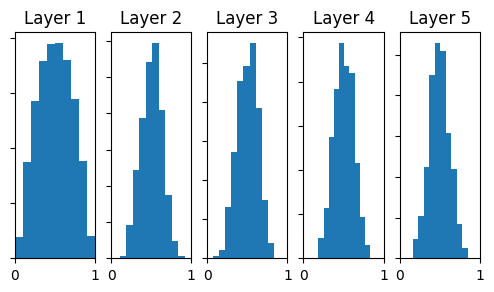
Now, let's experiment with the real world data and see what happens
Data: MNIST, \(x \in \mathbb{R}^{784}\)
Model: FFNN with three hidden layers
Loss: Cross entropy
Optimizer: Mini-Batch GD
Batch size: 256
Activation: tanh
W = np.random.randn(500,500)/ sqrt(fan_in)However this does not work for ReLU neurons
Why ?
Intuition: He et.al. argue that a factor of 2 is needed when dealing with ReLU Neurons
Intuitively this happens because the range of ReLU neurons is restricted only to the positive half of the space

380 iterations
30 iterations/s
Indeed when we account for this factor of 2 we see better performance
W = np.random.randn(fan_in,fan_out)/np.sqrt(fan_in/2)
Module 7.5 : Batch Normalization
Mitesh M. Khapra
AI4Bharat, Department of Computer
Science and Engineering, IIT Madras
We will now see a method called batch normalization which allows us to be less careful about initialization
To understand the intuition behind Batch Normalization let us consider a deep network
Let us focus on the learning process for the weights between these two layers
Typically we use mini-batch algorithms
What would happen if there is a constant change in the distribution of \(h_3\)
In other words what would happen if across minibatches the distribution of \(h_3\) keeps changing
Would the learning process be easy or hard?
It would help if the pre-activations at each layer were unit gaussians

Why not explicitly ensure this by standardizing the pre-activation ?

But how do we compute \(E[s_{ik}])\) and \(Var[s_{ik}]\)?
We compute it from a mini-batch
Thus we are explicitly ensuring that the distribution of the inputs at different layers does not change across batches
This is what the deep network will look like with Batch Normalization
Is this legal ?
tanh
tanh
tanh
BN
BN
Yes, it is because just as the tanh layer is differentiable, the Batch Normalization layer is also differentiable
Hence we can backpropagate through this layer
Catch: Do we necessarily want to force a unit gaussian input to the tanh layer?
tanh
tanh
tanh
BN
BN
Why not let the network learn what is best for it?
After the Batch Normalization step add the following step:
What happens if the network learns:
\( \gamma^k \)and \(\beta^k\) are additional parameters of the network.
We will recover \(s_{ik} \)
In other words by adjusting these additional parameters the network can learn to recover \(s_{ik}\) if that is more favourable
Accumulated activations for \(m\) training samples
Let \(x_i^j\) denotes the activation of \(i^{th}\) neuron for \(j^{th}\) training sample

We have three variables \(l,i, j\) involved in the statistics computation. Let's visualize these as three axes that form a cube.
Let us associate an accumulator with \(l^{th}\) layer that stores the activations of batch inputs.
Accumulated activations for \(m\) training samples
Let \(x_i^j\) denotes the activation of \(i^{th}\) neuron for \(j^{th}\) training sample
We have three variables \(l,i, j\) involved in the statistics computation. Let's visualize these as three axes that form a cube.
Let us associate an accumulator with \(l^{th}\) layer that stores the activations of batch inputs.
We will now compare the performance with and without batch normalization on MNIST data using 7 layers....
Without Batch Normalization
With Batch Normalization


Blue: Without BN
Red: With BN
Sigmoid Activation, w=0.1*np.random.randn()
Limitations of Batch Normalization
The accuracy of estimation of mean and variance depends on the size of \(m\). So using , due to memory constraint for data like image and videos, a smaller size of \(m\) results in high error.
Because of this, we can't use a batch size of 1 at all (i.e, it won't make any difference, \(\mu_i=x_i,\sigma_i=0\))
Many alternatives were proposed like Group normalization, Instance Normalization which are domain specific. However, the simplest one among them is called Layer Normalization.
Other than this limitation, it was also empirically found that the naive use of BN leads to performance degradation in NLP tasks (source).
There was also a systematic study that validated the statement and proposed a new normalization technique (by modifying BN) called powerNorm.
Ironically, it was later found that the Batch Normalization helps in better training not because it reduces internal covariate shift (i.e., reduce the fluctuations in the distribution of activations because of continues parameter update)
Instead, it smoothens the loss surface to help the optimization algorithm to reach the local minimum quickly.

Layer Normalization
