CS7015 (Deep Learning) : Lecture 6

So far, we have focused on minimizing the objective function using a variety of optimization algorithms

Therefore, they are called over-parameterized models

Over-parameterized models are prone to a phenomenon called over-fitting

To understand this, let's start with bias and variance of a model with respect to its capacity

Let us consider the problem of fitting a curve through a given set of points

We consider two models :

\(Simple \)

(\(degree:1\))

\(y = \hat {f}(x) = w_1x +w_0\)

\(Complex \)

(\(degree:25\))

Note that in both cases we are making an assumption about how \(y\) is related to \(x\). We have no idea about the true relation \(f(x)\)

The points were drawn from a sinusoidal function (the true \(f(x)\)) 

The training data consists of 500 points

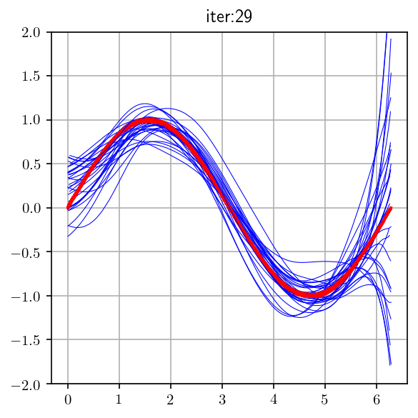
We sampled 500 points from the training data and train a simple and a complex model 

We repeat the process ‘k’ times to train multiple models (each model sees a different sample of the training data)

We make a few observations from these plots

Simple models trained on different samples of the data do not differ much from each other

However they are very far from the true sinusoidal curve (under fitting)

On the other hand, complex models trained on different samples of the data are very different from each other (high variance)

Let \(f(x)\) be the true model (sinusoidal in this case) and \(\hat {f}(x)\) be our estimate of the model (simple or complex, in this case) then,

Bias \(\hat {f}(x)\) \(= E\) [\(\hat {f}(x)\)] \(- f(x)\) 

Green Line: Average value of \(\hat {f}(x)\)for the simple model

Blue Curve: Average value of \(\hat {f}(x)\) for the complex model

Red Curve: True model (\(f(x))\)

\(E\) [\(\hat {f}(x)\)] is the average (or expected) value of the model

We can see that for the simple model the average value (green line) is very far from the true value \(f(x)\) (sinusoidal function)

Mathematically, this means that the simple model has a high bias

On the other hand, the complex model has a low bias

We now define,

Variance \(\hat{f}(x) = E\bigg[(\hat{f}(x) - E[\hat{f}(x)])^2\bigg]\) (Standard definition from statistics)

Roughly speaking it tells us how much the different \(\hat {f}(x)\)’s (trained on different samples of the data) differ from each other)

It is clear that the simple model has a low variance whereas the complex model has a high variance

In summary (informally)

Simple model: high bias, low variance

Complex model: low bias, high variance

There is always a trade-off between the bias and variance

Both bias and variance contribute to the mean square error. Let us see how

Consider a new point (\(x, y)\) which was not seen during training

If we use the model  \(\hat {f}(x)\) to predict the value of \(y\) then the mean square error is given by

\(E[(y −\) \(\hat {f}(x))^2 ]\)

(average square error in predicting \(y\) for many such unseen points)

We can show that

See proof here

However, at test time we are interested in evaluating the model on a validation (unseen) set which was not used for training

This gives rise to the following two entities of interest:

\(train_{err}\) (say, mean square error)

\(test_{err}\) (say, mean square error)

Typically these errors exhibit the trend shown in the adjacent figure

model complexity

High bias

High variance

Sweet spot-
-perfect tradeoff
-ideal model
complexity

Let there be \(n\) training points and \(m\) test (validation) points

\(train_{err}\) = \(\frac {1}{n} \displaystyle \sum_{i=1}^n  (y_{i} - \hat f {(x_i)})^2\)

\(test_{err} =\) \(\frac {1}{m} \displaystyle \sum_{i=n+1}^{n+m}  (y_{i} - \hat f {(x_i)})^2\)

As the model complexity increases \(train_{err}\) becomes overly optimistic and gives us a wrong picture of how close \(\hat f\) is to \(f\)

The validation error gives the real picture of how close \(\hat f\) is to \(f\)

We will concretize this intuition mathematically now and eventually show how to account for the optimism in the training error

Let D=\({\{x_i , y_i\}} ^{m+n}_ {i=1}\)

We know that some true function exists, s.t., 

\(y = f(x) + ε\)

which means that \(y_i\) is related to \(x_i\) by some true function \(f\) but there is also some noise \(ε\) in the relation

For simplicity, we assume

\(ε ∼ N (0, σ^2 )\)

and of course we do not know \(f\)

Further we use \(\hat f\) to approximate \(f\) and estimate the parameters using T \(\subset\)  D such that

\(y = \hat f(x)\)

We are interested in knowing

\(E[( \hat f(x) − f(x))^2 ]\)

but we cannot estimate this directly because we do not know \(f\)

We will see how to estimate this empirically using the observation \(y_i\) & prediction \(\hat y_i\)

\(E[( \hat y − y)^ 2 ]\)

\(= E[( \hat f(x) − f(x) − ε)^ 2 ]\)            (\(y = f(x) + ε)\)

\(= E[( \hat f(x) − f(x))^2 − 2ε( \hat f(x) − f(x)) + ε^2 ]\)

\(= E[( \hat f(x) − f(x))^2 ] − 2E[ε( \hat f(x) − f(x))] + E[ε^2 ]\)

\(∴ E[( \hat f(x) − f(x))^2 ] = E[( \hat y − y)^2 ] − E[ε^2 ] + 2E[ ε( \hat f(x) − f(x)) ]\)

\(E[( \hat y_i − y_i)^ 2 ]\)

\(= E[( \hat f(x_i) − f(x_i) − ε_i)^ 2 ]\)            (\(y_i = f(x_i) + ε_i)\)

\(= E[( \hat f(x_i) − f(x_i))^2 − 2ε_i( \hat f(x_i) − f(x_i)) + ε^2_i ]\)

\(= E[( \hat f(x_i) − f(x_i))^2 ] − 2E[ε_i( \hat f(x_i) − f(x_i))] + E[ε^2_i ]\)

\(∴ E[( \hat f(x_i) − f(x_i))^2 ] = E[( \hat y_i − y_i)^2 ] − E[ε^2_i ] + 2E[ ε_i( \hat f(x_i) − f(x_i)) ]\)

Suppose we have observed the goals scored (\(z)\) in \(k\) matches as

\(z_1\) = 2, \(z_2\) = 1, \(z_3\) = 0, ... \(z_k\) = 2

Now we can empirically estimate \(E[z]\) i.e. the expected number of goals scored as

\(E[z] = \frac {1}{k} \displaystyle \sum_{i=1}^k z_i\)

Analogy with our derivation: We have a certain number of observations \(y_i\) & predictions \(\hat y_i\) using which we can estimate

                           \(E[( \hat y − y)^2 ] =\)

\(\frac {1}{m} \displaystyle \sum_{i=1}^m (\hat y_i - y_i)^2\)

\(E[( \hat f(x) − f(x))^2 ] = E[( \hat y − y)^2 ] − E[ε^2] + 2E[ ε( \hat f(x) − f(x)) ]\)

We can empirically evaluate R.H.S using training observations or test observations

              Case 1: Using test observations

\(\underbrace {E[( \hat f(x) − f(x))^2 ]}_{true \space error} \)

\(= \underbrace {\frac{1}{m} \displaystyle \sum_{i=n+1}^{n+m}  (\hat y_i - y_{i}) ^2}_ {empirical \space estimation \space of \space error}  -\)

\(\underbrace {\sigma^2 }_ {small \space constant}   +\)

\(\underbrace{2  E[ ε( \hat f(x) − f(x))]}_ {= \space covariance (\space ε, ( \hat f(x) − f(x))}\)

\(∵\) covariance \((X, Y )\)

\(= E[(X − \mu_X)(Y − \mu_Y )]\)

\(= E[(X)(Y − \mu_Y )](\)if \(\mu_X = E[X] = 0)\)

\(= E[XY ] − E[X{\mu_Y}]\)

\(= E[XY ] − \mu_Y E[X]\)

\(= E[XY ]\)

\(\underbrace {E[( \hat f(x) − f(x))^2 ]}_{true \space error} \)

None of the test observations participated in the estimation of \(\hat f(x)\) [the parameters of \(\hat f(x)\) were estimated only using training data]

\(\because ε = ( y − f(x))\)

\(∴ E[ε\space · ( \hat f(x) − f(x))]\)

\(= E[ε ] · E[ \hat f(x) − f(x))]\)

\(= 0 \space · \space E[ \hat f(x) − f(x))]\)

\(= 0\)

∴ true error = empirical test error + small constant

Hence, we should always use a validation set(independent of the training set) to estimate the error M

\(∴ ε ⊥ ( \hat f(x) − f(x))\)

\(∴ (y - f(x) )⊥ ( \hat f(x) − f(x))\)

Case 2: Using training observations

\(\underbrace {E[( \hat f(x) − f(x))^2 ]}_{true \space error} \)

Now, \(y-f(x) \space \cancel{⊥} \space \hat f(x) - f(x)\) because the training data was used for estimating the parameters of \(\hat f(x)\)

\(\cancel{=} \space E[ε ] \space·\space E[ \hat f(x) − f(x))]\)

Hence, the empirical train error is smaller than the true error and does not give a true picture of the error

But how is this related to model complexity? Let us see

\(\cancel{=} \space 0\)

\(\space E[ε · \hat f(x) − f(x))]\)

Using Stein’s Lemma (and some trickery) we can show that

\(\frac{1}{n} \displaystyle \sum_{i=1}^{n} ε_i( \hat f(x_i) − f(x_i)) = \frac {\sigma^2}{n}\displaystyle \sum_{i=1}^{n} \frac{∂ \hat f(x_i)} {∂y_i}\)

When will \( \frac{∂ \hat f(x_i)} {∂y_i}\) be high? When a small change in the observation causes a large change in the estimation(\(\hat f\))

Can you link this to model complexity?

Yes, indeed a complex model will be more sensitive to changes in observations whereas a simple model will be less sensitive to changes in observations

Hence, we can say that true error \(=\) empirical train error \(+\) small constant \(+\) \(Ω\)(model complexity)

Let us verify that indeed a complex model is more sensitive to minor changes in the data

We have fitted a simple and complex model for some given data

We now change one of these data points

The simple model does not change much as compared to the complex model 

Hence while training, instead of minimizing the training error \(\mathscr {L}_{train} (\theta)\) we should minimize

min\(_{w.r.t \space \theta}\) \(\space \mathscr {L}_{train} (\theta)+ Ω(θ) = \mathscr {L}(\theta)\)

Where \(Ω(\theta)\) would be high for complex models and small for simple models

\(Ω(\theta)\) acts as an approximate for \(\frac {\sigma^2}{n}\textstyle \sum_{i=1}^{n} \frac{∂ \hat f(x_i)} {∂y_i}\)

This is the basis for all regularization methods

We can show that \(l_1\) regularization, \(l_2\) regularization, early stopping and injecting noise in input are all instances of this form of regularization.

Why do we care about this bias variance tradeoff and model complexity?

Deep Neural networks are highly complex models.

Many parameters, many non-linearities. 

It is easy for them to overfit and drive training error to 0. 

Hence we need some form of regularization. 

\(l_2\) regularization

Dataset augmentation

Parameter Sharing and tying

Adding Noise to the inputs 

Adding Noise to the outputs 

Early stopping

Ensemble methods

Dropout

For \(l_2\) regularization we have,

\(\widetilde{\mathscr {L}}(w) = \mathscr {L}(w) + \frac{\alpha}{2}\|w\|^2 \)

For SGD (or its variants), we are interested in

\(\nabla \widetilde{\mathscr {L}}(w) = \nabla \mathscr {L}(w) + \alpha w \)

Update rule:

\(w_{t+1} = w_t - \eta \nabla \mathscr {L}(w_t) - \eta \alpha w_t \)

Requires a very small modification to the code

Let us see the geometric interpretation of this

Assume \(w^∗\) is the optimal solution for \(\mathscr {L}(w)\)  [not \(\widetilde{ \mathscr {L}}(w)\)] i.e. the solution in the absence of regularization (\(w^∗\) optimal → \(\nabla \mathscr {L}(w^*)=\) 0)

Consider \(u = w − w^∗\) . Using Taylor series approximation (upto \(2^{nd}\) order)

\(\mathscr {L}(w^* + u) = \mathscr {L}(w^*) + u^T \nabla \mathscr {L}(w^*) + \dfrac{1}{2}u^THu\)

\(\mathscr {L}(w) = \mathscr {L}(w^*) + (w - w^*)^T \nabla \mathscr {L}(w^*) + \dfrac{1}{2}(w - w^*)^TH(w - w^*)\)

\(= \mathscr {L}(w^*) + \dfrac{1}{2}(w - w^*)^TH(w - w^*)\)                \((∵ \nabla \mathscr {L}(w^*) = 0)\)

\(\nabla \mathscr {L}(w)= \nabla \mathscr {L}(w^*) + H(w - w^*)\)  

\(= H(w - w^*)\)  

Now,

\(\nabla \widetilde{\mathscr {L}}(w) = \nabla \mathscr{L}(w) + \alpha w\)

\(= H(w - w^*) + \alpha w\)

Let \(\widetilde w\) be the optimal solution for \(\widetilde{\mathscr{L}}(w)\) [i.e regularized loss]

\(∵ \nabla \widetilde{\mathscr {L}}(\widetilde w) = 0\)

\(H( \widetilde{w} - w^*) + \alpha \widetilde w = 0\)

\(∴ (H + \alpha \mathbb I) \widetilde{w} = H w^* \)

\(∴ \widetilde w = (H + \alpha \mathbb I)^{-1} H w^* \)

Notice that if \(\alpha → 0\) then \(\widetilde w → w^∗\) [no regularization]

But we are interested in the case when \(\alpha \space \cancel{=} \space 0\)

Let us analyse the case when \(\alpha \space \cancel{=} \space 0\)

If H is symmetric Positive Semi Definite

\(H = Q \Lambda Q^T\)  [\(Q\) is orthogonal, \(QQ^T = Q^TQ = \mathbb I\)]

\(∴ \widetilde w = (H + \alpha \mathbb I)^{-1} H w^* \)

\(= (Q \Lambda Q^T + \alpha \mathbb I)^{-1} Q \Lambda Q^T w^*\)

\(= (Q \Lambda Q^T + \alpha Q \mathbb I Q^T)^{-1} Q \Lambda Q^T w^*\)

\(= [Q (\Lambda+ \alpha \mathbb I) Q^T]^{-1} Q \Lambda Q^T w^*\)

\(= Q^{T^{-1}} (\Lambda+ \alpha \mathbb I)^{-1} Q^{-1} Q \Lambda Q^T w^*\)

\(= Q (\Lambda+ \alpha \mathbb I)^{-1} \Lambda Q^T w^*\)               (\(∵ Q^{T^{-1}} = Q\))

\(∴ \widetilde w = (QDQ)^{T} w^* \)

where \(D = (\Lambda + \alpha \mathbb I)^{−1} \Lambda\), is a diagonal matrix which we will see in more detail soon

\(∴ \widetilde w = Q(\Lambda + \alpha \mathbb I)^{−1} \Lambda Q^T w^* \)

 \(= QDQ^T w^* \)

So what is happening here?

\(w^∗\) first gets rotated by \(Q^T\) to give \(Q^T w^∗\)

However if \(\alpha = 0\) then \(Q\) rotates \(Q^T w^∗\) back to give \(w^∗\)

If \(\alpha \space \cancel{=} \space 0\) then let us see what \(D\) looks like

\((\Lambda + \alpha \mathbb I)^{−1} =\)

\(D = (\Lambda + \alpha \mathbb I)^{−1} \Lambda\)

\((\Lambda + \alpha \mathbb I)^{−1} \Lambda =\) 

So what is happening now?

\(∴ \widetilde w = Q(\Lambda + \alpha \mathbb I)^{−1} \Lambda Q^T w^* \)

 \(= QDQ^T w^* \)

Each element \(i\) of \(Q^T w^∗\) gets scaled by \(\frac {\lambda_i} {\lambda_i + a}\) before it is rotated back by \(Q\) 

if \(\lambda_i >> \alpha\) then \(\frac {\lambda_i} {\lambda_i + a} = 1\)

if \(\lambda_i << \alpha\) then \(\frac {\lambda_i} {\lambda_i + a} = 0\)

Thus only significant directions (larger eigen values) will be retained.

\((\Lambda + \alpha \mathbb I)^{−1} =\)

\(D = (\Lambda + \alpha \mathbb I)^{−1} \Lambda\)

\((\Lambda + \alpha \mathbb I)^{−1} \Lambda =\) 

Effective parameters \( = \displaystyle \sum_{i=1}^{n} \frac{\lambda_i}{\lambda_i + a} < n \)

The weight vector\((w^∗)\) is getting rotated to (\(\widetilde w)\)

All of its elements are shrinking but some are shrinking more than the others

This ensures that only important features are given high weights

[given training data]

label = 2

[augmented data = created using some knowledge of the
task]

We exploit the fact that
certain transformations
to the image do not
change the label of the
image.

Works well for image classification / object recognition tasks

Also shown to work well for speech

For some tasks it may not be clear how to generate such data

Used in CNNs

Same filter applied at different positions of the image 

Or same weight matrix acts on different input neurons

Typically used in autoencoders.

The encoder and decoder weights are tied.

We saw this in Autoencoder

We can show that for a simple input output neural network, adding Gaussian noise to the input is equivalent to weight decay (L2 regularisation)

Can be viewed as data augmentation

\(\widetilde {x}_i = x_i + ε_i\)

\(\widehat y = \displaystyle \sum_{i=1}^{n} w_i x_i\)

\(= \displaystyle \sum_{i=1}^{n} w_i x_i + \displaystyle \sum_{i=1}^{n} w_i ε_i\)

\(= \widehat y + \displaystyle \sum_{i=1}^{n} w_i ε_i\)

We are interested in \(E[(\widetilde y - y)^2]\)

\(E[(\widetilde y - y)^2] = E \Biggl [(\hat y + \displaystyle \sum_{i=1}^{n} w_i ε_i -y)^2 \Biggl]  \)  

\(= E \Biggl [\bigg(\big(\hat y - y \big) + \big(\displaystyle \sum_{i=1}^{n} w_i ε_i )\bigg)^2 \Biggl]  \)  

\(= E  [(\hat y - y)^2] + E \Big[2(\hat y - y) \displaystyle \sum_{i=1}^{n} w_i ε_i\Big] + E \Big[ \big(\displaystyle \sum_{i=1}^{n} w_i ε_i \big)^2 \Big]  \)  

\(= E  [(\hat y - y)^2] + 0 + E \Big[ \displaystyle \sum_{i=1}^{n} {w_i}^2 {ε_i}^2 \Big]  \)  

(\(∵ ε_i\) is independent of \(ε_j\) and \(ε_i\) is independent of \((\hat y-y)\))

\(= (E  \Big[(\hat y - y)^2\Big] + \sigma^2  \displaystyle \sum_{i=1}^{n} {w_i}^2\)    (same as \(L_2\) norm penalty)

\(\tilde y = \displaystyle \sum_{i=1}^{n} w_i \widetilde{x}_i\)

minimize : \( \displaystyle \sum_{i=0}^{9} p_i \space log \space q_i\)

true distribution : \(p = {0, 0, 1, 0, 0, 0, 0, 0, 0, 0}\)

estimated distribution : \(q\)

Do not trust the true labels, they may be noisy

Instead, use soft targets

\(ε =\) small positive constant

minimize : \( \displaystyle \sum_{i=0}^{9} p_i \space log \space q_i\)

true distribution + noise : \(p =\{\frac{\varepsilon}{9}, \frac{\varepsilon}{9}, 1 - \varepsilon, \frac{\varepsilon}{9}, ... \}  \)

estimated distribution : \(q\)

Have a patience parameter \(p\)

If you are at step \(k\) and there was no improvement in validation error in the previous \(p\) steps then stop training and return the model stored at step \(k − p\)

Basically, stop the training early before it drives the training error to 0 and blows up the validation error

Can be used even with other regularizers (such as \(l_2\)) 

How does it act as a regularizer ?

We will first see an intuitive explanation and then a mathematical analysis

\(w_{t+1} = w_t - \eta \nabla w_t\)

\(= w_0 - \eta \displaystyle \sum_{i=1}^{t} \nabla w_i \)

Let \(τ\) be the maximum value of \( \nabla w_i\) then

\(\mid w_{t+1} - w_0 \mid \space \leq \eta t \mid τ \mid\)

Thus, \(t\) controls how far \(w_t\) can go from the initial \(w_0\)

In other words it controls the space of exploration 

Recall that the Taylor series approximation for \(\mathscr{L} (w)\) is

\(\mathscr{L}(w) = \mathscr{L}(w^*) + (w - w^*)^T \nabla \mathscr{L}(w^*) + \dfrac{1}{2} (w - w^*)^T H(w - w^*) \)

\(= \mathscr{L}(w^*) + \dfrac{1}{2} (w - w^*)^T H(w - w^*) \)             \([ w^* \space is \space optimal \space so \space \nabla \mathscr{L} (w^∗) \space is \space 0 ]\)

\( \nabla (\mathscr{L} (w^∗))=  H(w - w^*) \)

Now the SGD update rule is:

\(w_t = w_{t-1} - \eta \nabla \mathscr{L} (w_{t-1})\)

\(= w_{t-1} - \eta H (w_{t-1} - w^*)\)

\(= (I - \eta H)w_{t-1} + \eta H w^*\)

\(w_t = (I - \eta H)w_{t-1} + \eta H w^*\)

Using EVD of \(H\) as \(H\) = \(Q \Lambda Q^T\) , we get:

                               \(w_t = (I - \eta Q \Lambda Q^T)w_{t-1} + \eta Q \Lambda Q^T w^*\)

If we start with \(w_0 = 0\) then we can show that (See Appendix)

                               \(w_t = Q[I - (I - \varepsilon \Lambda)^t] Q^T w^*\)

Compare this with the expression we had for optimum \(\tilde W\) with \(L_2\) regularization

                               \(\tilde w = Q[I - (\Lambda + \alpha I)^{-1} \alpha] Q^T w^*\)

We observe that \(w_t = \tilde w\), if we choose \(ε,t\) and \(\alpha\) such that

                               \((I - \varepsilon \Lambda)^t =  (\Lambda + \alpha I)^{-1} \alpha \)

Early stopping only allows \(t\) updates to the parameters.

If a parameter \(w\) corresponds to a dimension which is important for the loss \(\mathscr{L} (\theta)\) then \(\frac {∂\mathscr{L} (\theta)}{∂w}\) will be large

However if a parameter is not important (\(\frac {∂\mathscr{L} (\theta)}{∂w}\) is small) then its updates will be small and the parameter will not be able to grow large in '\(t\)'  steps 

Early stopping will thus effectively shrink the parameters corresponding to less important directions (same as weight decay).

Combine the output of different models to reduce generalization error

The models can correspond to different classifiers

It could be different instances of the same classifier trained with:

different hyperparameters

different features 

different samples of the training data

Bagging: form an ensemble using different instances of the same classifier

From a given dataset, construct multiple training sets by sampling with replacement \((T_1, T_2, ..., T_k)\)

Train \(i^{th}\) instance of the classifier using training set \(T_i\)

Each model trained with a different sample of the data (sampling with replacement)

When would bagging work?

Consider a set of k LR models

Suppose that each model makes an error \(\varepsilon_i\) on a test example

The error made by the average prediction of all the models is \(\frac {1}{k} \textstyle \sum_{i} \varepsilon_i\)

Let \(\varepsilon_i\) be drawn from a zero mean multivariate normal distribution

\(Variance = E[\varepsilon_i^2] = V\)

\(Covariance = E[\varepsilon_i \varepsilon_j] = C\)

The expected squared error is :

\(mse = E[(\frac {1}{k} \textstyle \sum_{i} \varepsilon_i)^2]\)

\(= \frac {1}{k^2} E[ \displaystyle \sum_{i} \displaystyle \sum_{i = j} \varepsilon_i \varepsilon_j + \displaystyle \sum_{i} \displaystyle \sum_{i \cancel{=} j} \varepsilon_i \varepsilon_j ]\)

\(= \frac {1}{k^2} E[ \displaystyle \sum_{i} \varepsilon_i^2 + \displaystyle \sum_{i} \displaystyle \sum_{i \cancel{=} j} \varepsilon_i \varepsilon_j ]\)

\(= \frac {1}{k^2} (\displaystyle \sum_{i} E [\varepsilon_i^2] + \displaystyle \sum_{i} \displaystyle \sum_{i \cancel{=} j} E[\varepsilon_i \varepsilon_j ])\)

\(= \frac {1}{k^2} (kV+ k(k-1)C)\)

\(= \frac {1}{k}V + \dfrac{k-1}{k}C\)

When would bagging work?

If the errors of the model are perfectly correlated then \(V = C\) and \(mse = V\) [bagging does not help: the mse of the ensemble is as bad as the individual models] 

If the errors of the model are independent or uncorrelated then \(C = 0\) and the mse of the ensemble reduces to \(\frac{1}{k}V\)

\(mse = \frac {1}{k}V + \dfrac{k-1}{k}C\)

On average, the ensemble will perform at least as well as its individual members

Typically model averaging (bagging ensemble) always helps

Training several large neural networks for making an ensemble is prohibitively expensive

Option 1: Train several neural networks having different architectures(obviously expensive)

Option 2: Train multiple instances of the same network using different training samples (again expensive) 

Even if we manage to train with option 1 or option 2, combining several models at test time is infeasible in real time applications