Classification functions in sci-kit learn
Dr. Ashish Tendulkar
Machine Learning Practice
IIT Madras
- In this week, we will study sklearn functionality for implementing classification algorithms.
- We will cover sklearn APIs for
- Specific classification algorithms for least square classification, perceptron, and logistic regression classifier.
- with regularization
- multiclass, multilabel and multi-output setting
- Various classification metrics.
- Specific classification algorithms for least square classification, perceptron, and logistic regression classifier.
-
Cross validation and hyper parameter search for classification works exactly like how it works in regression setting.
- However there are a couple of CV strategies that are specific to classification
Part I: sklearn API for classification
- Logistic regression
- Perceptron
- Ridge classifier (for LSC)
- K-nearest neighbours (KNNs)
- Support vector machines (SVMs)
- Naive Bayes
There are broadly two types of APIs based on their functionality:
Specific
Generic
- SGD classifier
Uses gradient descent for opt
Specialized solvers for opt
Need to specify loss function
All sklearn estimators for classification implement a few common methods for model training, prediction and evaluation.
Model training
fit(X, y[, coef_init, intercept_init, …])
Prediction
predict(X)
decision_function(X)
predicts class label for samples
predicts confidence score for samples.
Evaluation
score(X, y[, sample_weight])
Return the mean accuracy on the given test data and labels.
There a few common miscellaneous methods as follows:
get_params([deep])
gets parameter for this estimator.
converts coefficient matrix to dense array format.
set_params(**params)
densify()
sparsify()
sets the parameters of this estimator.
converts coefficient matrix to sparse format.
Now let's study how to implement different classifiers with sklearn APIs.
Let's start with implementation of least square classification (LSC) with RidgeClassifier API.
Ridge classifier
- treated as multi-output regression
- predicted class corresponds to the output with the highest value
- classifier first converts binary targets to {-1, 1} and then treats the problem as a regression task, optimizing the objective of regressor:
Binary classification:
Multiclass classification:
- minimize a penalized residual sum of squares
-
\(\min\limits_\mathbf w ||\mathbf{Xw}-\mathbf{y}||_2^2 + \alpha ||\mathbf w||_2^2\)
- sklearn provides different solvers for this optimization
- sklearn uses \(\alpha\) to denote regularization rate
- predicted class corresponds to the sign of the regressor’s prediction
-
\(\min\limits_\mathbf w ||\mathbf{Xw}-\mathbf{y}||_2^2 + \alpha ||\mathbf w||_2^2\)
How to train a least square classifier?
Step 1: Instantiate a classification estimator without passing any arguments to it. This creates a ridge classifier object.
from sklearn.linear_model import RidgeClassifier
ridge_classifier = RidgeClassifier()
Step 2: Call fit method on ridge classifier object with training feature matrix and label vector as arguments.
Note: The model is fitted using X_train and y_train.
# Model training with feature matrix X_train and
# label vector or matrix y_train
ridge_classifier.fit(X_train, y_train)
How to set regularization rate in RidgeClassifier?
Set alpha to float value. The default value is 0.1.
- alpha should be positive.
- Larger alpha values specify stronger regularization.
from sklearn.linear_model import RidgeClassifier
ridge_classifier = RidgeClassifier(alpha=0.001)
How to solve optimization problem in RidgeClassifier?
Using one of the following solvers
svd
cholesky
sparse_cg
lsqr
sag , saga
uses a Singular Value Decomposition of the feature matrix to compute the Ridge coefficients.
lbfgs
uses scipy.linalg.solve function to obtain the closed-form solution
uses the conjugate gradient solver of scipy.sparse.linalg.cg .
uses the dedicated regularized least-squares routine scipy.sparse.linalg.lsqr and it is fastest.
uses a Stochastic Average Gradient descent iterative procedure
'saga' is unbiased and more flexible version of 'sag'
uses L-BFGS-B algorithm implemented in scipy.optimize.minimize .
can be used only when coefficients are forced to be positive.
Uses of solver in RidgeClassifier
- For large scale data, use '
sparse_cg' solver.
-
When both
n_samplesandn_featuresare large, use ‘sag’ or ‘saga’ solvers.-
Note that fast convergence is only guaranteed on features with approximately the same scale.
-
How to make RidgeClassifier select the solver automatically?
auto
chooses the solver automatically based on the type of data
ridge_classifier = RidgeClassifier(solver=auto) if solver == 'auto':
if return_intercept:
# only sag supports fitting intercept directly
solver = "sag"
elif not sparse.issparse(X):
solver = "cholesky"
else:
solver = "sparse_cg"Default choice for solver is auto .
If data is already centered, set fit_intercept as false, so that no intercept will be used in calculations.
Is intercept estimation necessary for RidgeClassifier?
ridge_classifier = RidgeClassifier(fit_intercept=True)Default:
How to make predictions on new data samples?
Use predict method to predict class labels for samples
# Predict labels for feature matrix X_test
y_pred = ridge_classifier.predict(X_test)
Other classifiers also use the same predict method.
Step 2: Call predict method on classifier object with feature matrix as an argument.
Step 1: Arrange data for prediction in a feature matrix of shape (#samples, #features) or in sparse matrix format.
RidgeClassifierCV implements RidgeClassifier with built-in cross validation.
Let's implement perceptron classifier with Perceptron API.
-
It is a simple classification algorithm suitable for large-scale learning.
Perceptron classification
-
Shares the same underlying implementation with
SGDClassifier
Perceptron uses SGD for training.
Perceptron()
SGDClassifier(loss="perceptron", eta0=1, learning_rate="constant", penalty=None)
How to implement perceptron classifier?
Step 1: Instantiate a Perceptron estimator without passing any arguments to it to create a classifier object.
from sklearn.linear_model import Perceptron
perceptron_classifier = Perceptron()
Step 2: Call fit method on perceptron estimator object with training feature matrix and label vector as arguments.
# Model training with feature matrix X_train and
# label vector or matrix y_train
perceptron_classifier.fit(X_train, y_train)
Perceptron can be further customized with the following parameters:
penalty
(default = 'l2')
alpha
(default = 0.0001)
l1_ratio
(default = 0.15)
fit_intercept
(default = True)
max_iter
(default = 1000)
tol
(default = 1e-3)
eta0
(default = 1)
early_stopping
(default = False)
validation_fraction
(default = 0.1)
n_iter_no_change
(default = 5)
- Perceptron classifier can be trained in an iterative manner with partial_fit method
- Perceptron classifier can be initialized to the weights of the previous run by specifying warm_start = True in the constructor.
Let's implement logistic regression classifier with LogisticRegression API.
LogisticRegression API
- Implements logistic regression classifier, which is also known by a few different names like logit regression, maximum entropy classifier (maxent) and log-linear classifier.
- This implementation can fit
- binary classification
- one-vs-rest (OVR)
- multinomial logistic regression
- Provision for \(\ell_1,\ell_2\) or elastic-net regularization
How to train a LogisticRegression classifier?
Step 1: Instantiate a classifier estimator without passing any arguments to it. This creates a logistic regression object.
from sklearn.linear_model import LogisticRegression
logit_classifier = LogisticRegression()
Step 2: Call fit method on logistic regression classifier object with training feature matrix and label vector as arguments
# Model training with feature matrix X_train and
# label vector or matrix y_train
logit_classifier.fit(X_train, y_train)
Logistic regression uses specific algorithms for solving the optimization problem in training. These algorithms are known as solvers.
The choice of the solver depends on the classification problem set up such as size of the dataset, number of features and labels.
How to select solvers for Logistic Regression classifier?
solver
- For small datasets, ‘liblinear’ is a good choice, whereas ‘sag’ and ‘saga ’ are faster for large ones.
- For multiclass problems, only ‘
newton-cg’, ‘sag’, ‘saga’ and ‘lbfgs’ handle multinomial loss. - ‘
liblinear’ is limited to one-versus-rest schemes
‘newton-cg ’
‘lbfgs ’
‘liblinear ’
‘sag
‘saga ’
logit_classifier = LogisticRegression(solver='lbfgs')- For unscaled datasets, ‘
liblinear', 'lbfgs' and 'newton-cg' are robust.
By default, logistic regression uses lbfgs solver.
How to add regularization in Logistic Regression classifier?
Regularization is applied by default because it improves numerical stability.
penalty
- \(l2\) - adds a L2 penalty term
- \(l1\) - adds a L1 penalty term
- elasticnet - both L1 and L2 penalty terms are added
- none - no penalty is added
logit_classifier = LogisticRegression(penalty='l2')By default, it uses L2 penalty.
- Not all the solvers supports all the penalties.
-
Select appropriate solver for the desired penalty.
-
L2 penalty is supported by all solvers
-
L1 penalty is supported only by a few solvers.
-
| Solver | Penalty |
|---|---|
‘newton-cg ’ |
[‘l2’, ‘none’] |
‘lbfgs ’ |
[‘l2’, ‘none’] |
‘liblinear’ |
[‘l1’, ‘l2’] |
‘sag’ |
[‘l2’, ‘none’] |
‘saga ’ |
[‘elasticnet’, ‘l1’, ‘l2’, ‘none’] |
How to control amount of regularization in logistic regression?
- sklearn implementation uses parameter C, which is inverse of regularization rate to control regularization.
- Recall
- C is specified in the constructor and must be positive
- Smaller value leads to stronger regularization.
- Larger value leads to weaker regularization.
LogisticRegression classifier has a class_weight parameter in its constructor.
What purpose does it serve?
Exercise: Read stack overflow discussion on this parameter.
- Handles class imbalanace with differential class weights.
- Mistakes in a class are penalized by the class weight.
- Higher value here would mean higher emphasis on the class.
This parameter is available in classifier estimators in sklearn.
LogisticRegressionCV implements logistic regression with in built cross validation support to find the best values of C and l1_ratio parameters according to the specified scoring attribute.
These classifiers can also be implemented with a generic SGDClassifier API by setting the loss parameter appropriately.
Let's study SGDClassifier API.
- SGD is a simple yet very efficient approach to fitting linear classifiers under convex loss functions
SGDClassifier
- This API uses SGD as an optimization technique and can be applied to build a variety of linear classifiers by adjusting the loss parameter.
-
Easily scales up to large scale problems with more than \(10^5\) training examples and \(10^5\) features. It also works with sparse machine learning problems
- Text classification and natural language processing
- It supports multi-class classification by combining multiple binary classifiers in a “one versus all” (OVA) scheme.
We need to set loss parameter appropriately to build train classifier of our interest with SGDClassifier
loss parameter
'hinge' - (soft-margin) linear Support Vector Machine
'modified_huber' - smoothed hinge loss brings tolerance to outliers as well as probability estimates
'log' - logistic regression
'squared_hinge' - like hinge but is quadratically penalized
'perceptron' - linear loss used by the perceptron algorithm
‘squared_error’, ‘huber’, ‘epsilon_insensitive’, or ‘squared_epsilon_insensitive’ - regression losses
By default SGDClassifier uses hinge loss and hence trains linear support vector machine classifier.
SGDClassifier(loss='log')
LogisticRegression(solver='sgd')
SGDClassifier(loss='hinge')
Linear Support vector machine
- An instance of SGDClassifier might have an equivalent estimator in the scikit-learn API.
How does SGDClassifier work?
- SGDClassifier implements a plain stochastic gradient descent learning routine.
- the gradient of the loss is estimated with one sample at a time and the model is updated along the way with a decreasing learning rate (or strength) schedule.
Advantages:
- Efficiency.
- Ease of implementation
Disadvantages:
- Requires a number of hyperparameters.
- Sensitive to feature scaling.
-
It is important
- to permute (shuffle) the training data before fitting the model.
- to standardize the features.
How to use SGDClassifier for training a classifer?
Step 1: Instantiate a SGDClassifer estimator by setting appropriate loss parameter to define classifier of interest. By default it uses hinge loss, which is used for training linear support vector machine.
from sklearn.linear_model import SGDClassifier
SGD_classifier = SGDClassifier(loss='log')
Step 2: Call fit method on SGD classifier object with training feature matrix and label vector as arguments.
# Model training with feature matrix X_train and
# label vector or matrix y_train
SGD_classifier.fit(X_train, y_train)
Here we have used `log` loss that defines a logistic regression classifier.
How to perform regularization in SGD classifier?
penalty
- \(l2\) - adds a L2 penalty term
- \(l1\) - adds a L1 penalty term
- elasticnet - Convex combination of L2 and L1
(1 - l1_ratio) * L2 + l1_ratio * L1
SGD_classifier = SGDClassifier(penalty='l2')(l1_ratio controls the convex combination of L1 and L2 penalty. default=0.15)
Default:
- Constant that multiplies the regularization term.
- Has float values and default = 0.0001
alpha
How to set maximum number of epochs for SGD Classifier?
SGD_classifier = SGDClassifier(max_iter=100)Default:
max_iter = 1000
The maximum number of passes over the training data (aka epochs) is an integer that can be set by the max_iter parameter.
Some common parameters between SGDClassifier and SGDRegressor
learning_rate
Stopping criteria
warm_start
‘constant’
‘optimal’
‘invscaling’
‘adaptive’
average
- SGDClassifier also supports averaged SGD (ASGD)
‘True’
‘False’
tol
n_iter_no_change
max_iter
early_stopping
validation_fraction
Summary
We learnt how to implement the following classifiers with sklearn APIs:
- Least square classification (RidgeClassifier)
- Perceptron (Perceptron)
- Logistic regression (LogisticRegression)
Alternatively we can use SGDClassifier with appropriate loss setting for implementing these classifiers:
- loss = `log` for logistic regression
- loss = `perceptron` for perceptron
- loss = `squared_error` for least square classification
Classification estimators implements a few common methods like fit, score, decision_function, and predict.
- These estimators can be readily used in multiclass setting.
- They support regularized loss function optimization.
- All classification estimators have ability to deal with class imbalance through class_weight parameter in the constructor.
Part II: Multi-learning classification set up
Let's extend these classifiers to multi-learning (multi-class, multi-label & multi-output) settings.
Basics of multiclass, multilabel and multioutput classification
- Multiclass classification has exactly one output label and the total number of labels > 2.
- For more than one output, there are two types of classification models:
Multilabel
total #labels = 2
Multiclass multioutput
total #labels > 2
We will refer both these models as multi-label classification models, where # of output labels > 1.
Multiclass, multilabel, multioutput problems are referred to as multi-learning problems.
Multiclass classification
(sklearn.multiclass)
Multilabel classification
(sklearn.multioutput)
problem types
meta-estimators
OneVsOneClassifier
OneVsRestClassifier
OutputCodeClassifier
MultiOutputClassifier
ClassifierChain
- sklearn provides a bunch of meta-estimators, which extend the functionality of base estimators to support multi-learning problems.
- The meta-estimators transform the multi-learning problem into a set of simpler problems and fit one estimator per problem.
- Many sklearn estimators have built-in support for multi-learning problems.
- Meta-estimators are not needed for such estimators, however meta-estimators can be used in case we want to use these base estimators with strategies beyond the built-in ones.
Inherently multiclass
Multiclass as OVO
Multiclass as OVR
Multilabel
Inherently multiclass
Multilabel
LogisticRegression (multi_class = 'multinomial')
RidgeClassifier
LogisticRegressionCV (multi_class = 'multinomial')
RidgeClassifierCV
Multiclass as OVR
Perceptron
LogisticRegression (multi_class = 'ovr')
SGDClassifier
LogisticRegressionCV (multi_class = 'ovr')
RidgeClassifier
RidgeClassifierCV
First we will study multiclass APIs in sklearn.
Multi-class classification
- Classification task with more than two classes.
- Each example is labeled with exactly one class
In Iris dataset,
- There are three class labels: setosa, versicolor and virginica.
- Each example has exactly one label of the three available class labels.
- Thus, this is an instance of a multi-class classification.
In MNIST digit recognition dataset,
- There are 10 class labels: 0, 1, 2, 3, 4, 5, 6, 7, 8, 9.
- Each example has exactly one label of the 10 available class labels.
- Thus, this is an instance of a multi-class classification.
How to represent class labels in multi-class setup?
- Use LabelBinarizer transformation to convert the class label to multi-class format.
- Each example is marked with a single label out of k labels. The shape of label vector is \((n, 1)\).
- The resulting label vector has shape of \((n, k)\).
from sklearn.preprocessing import LabelBinarizer
y = np.array(['apple', 'pear', 'apple', 'orange'])
y_dense = LabelBinarizer().fit_transform(y)
[[1 0 0] [0 0 1] [1 0 0] [0 1 0]]
Let's say, you are given labels as part of the training set, how do we check if they are is suitable for multi-class classification?
- Use type_of_target to determine the type of the label.
from sklearn.utils.multiclass import type_of_target
type_of_target(y)- In case, \(y\) is a vector with more than two discrete values, type_of_target returns multiclass.
type_of_target can determine different types of multi-learning targets.
target_type
‘multiclass’
‘multiclass-multioutput’
‘unknown’
y
- contains more than two discrete values
- not a sequence of sequences
- 1d or a column vector
- array-like but none of the above, such as a 3d array,
- sequence of sequences, or an array of non-sequence objects.
- 2d array that contains more than two discrete values
- not a sequence of sequences
- dimensions are of size > 1
‘multilabel-indicator’
- label indicator matrix
- an array of two dimensions with at least two columns, and at most 2 unique values.
Examples
>>> type_of_target([1, 0, 2])
'multiclass'
>>> type_of_target([1.0, 0.0, 3.0])
'multiclass'
>>> type_of_target(['a', 'b', 'c'])
'multiclass'
>>> type_of_target(np.array([[1, 2], [3, 1]]))
'multiclass-multioutput'multiclass
multiclass-multioutput
multilabel-indicator
type_of_target(np.array([[0, 1], [1, 1]]))
'multilabel-indicator'
>>> type_of_target([[1, 2]])
'multilabel-indicator'
Apart from these, there are three more types, type_of_target can determine targets corresponding to regression and binary classification.
- continuous - regression target
- continuous-multioutput - multi-output target
- binary - classification
All classifiers in scikit-learn perform multiclass classification out-of-the-box.
- Use sklearn.multiclass module only when you want to experiment with different multiclass strategies.
- Using different multi-class strategy than the one implemented by default may affect performance of classifier in terms of either generalization error or computational resource requirement.
What are different multi-class classification strategies implemented in sklearn?
- One-vs-all or one-vs-rest (OVR)
- One-vs-One (OVA)
- OVR is implemented by OneVsRestClassifier API.
- OVA is implemented by OneVsOneClassifier API.
OVR - OneVsRestClassifier
- Fits one classifier per class \(c\) - \(c \text{ vs } \text{ not }c\).
- This approach is computationally efficient and requires only \(k\) classifiers.
- The resulting model is interpretable.
OneVsRest classifier also supports multilabel classification. We need to supply labels as indicator matrix of shape \((n, k)\).
from sklearn.multiclass import OneVsRestClassifier
OneVsRestClassifier(LinearSVC(random_state=0)).fit(X, y)- We need to supply estimator as an argument in the constructor.
- Support methods like other classifiers - fit, predict, predict_proba, partial_fit.
OVA - OneVsOneClassifier
- Fits one classifier per pair of classes. Total classifiers = \(k \choose 2\).
- Predicts class that receives maximum votes.
- The tie among classes is broken by selecting the class with the highest aggregate classification confidence.
OneVsOne classifier processes subset of data at a time and is useful in cases where the classifier does not scale with the data.
from sklearn.multiclass import OneVsOneClassifier
OneVsOneClassifier(LinearSVC(random_state=0)).fit(X, y)- We need to supply estimator as an argument in the constructor.
- Support methods like other classifiers - fit, predict, predict_proba, partial_fit.
What is the difference between OVR and OVA?
OneVsRestClassifier
OneVsOneClassifier
- Fits one classifier per class.
- For each classifier, the class is fitted against all the other classes.
-
Fits one classifier per pair of classes.
-
At prediction time, the class which received the most votes is selected.
Now we will learn how to perform multilabel and multi-output classification.
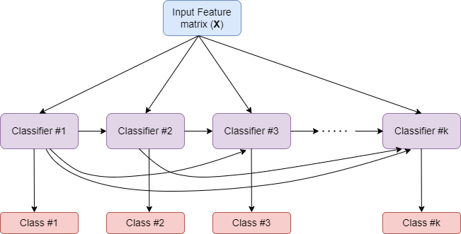
How MultiOutputClassifier works?
- Strategy consists of fitting one classifier per target.
- Allows multiple target variable classifications.
Input Feature Matrix (X)
Classifier #1
Classifier #2
Classifier #k
Class #1
Class #2
Class #k
How ClassifierChain works?
- A multi-label model that arranges binary classifiers into a chain.
- Way of combining a number of binary classifiers into a single multi-label model.
Comparison of MultiOutputClassifier and ClassifierChain
MultiOutputClassifier
ClassifierChain
- Allows multiple target variable classifications.
- Able to estimate a series of target functions that are trained on a single predictor matrix to predict a series of responses.
- For a multi-label classification problem with \(k\) classes, \(k\) binary classifiers are assigned an integer between 0 and \(k-1\).
- These integers define the order of models in the chain.
- Capable of exploiting correlations among targets.
Summary
- Different types of multi-learning setups: multi-class, multi-label, multi-output.
- type_of_target to determine the nature of supplied labels.
- Meta-estimators:
- multi-class: One-vs-rest, one-vs-one
- multi-label: Classifier chain and multi-output classifier
Evaluating Classifiers
So far we learnt how to train classifiers for binary, multi-class and multi-label/output cases.
We will learn how to evaluate these classifiers with different scoring functions and with cross-validation.
We will also study how to set hyper-parameters for classifiers.
Many cross-validation and HPT methods discussed in the regression context are also applicable in classifiers.
- We will not repeat that discussion in this topic.
- Instead we will focus on only additional methods that are specific to classifiers.
There may be issues like class imbalance in classification, which tend to impact the cross validation folds.
The overall class distribution and the ones in folds may be different and this has implications in effective model training.
sklearn.model_selection module provides three stratified APIs to create folds such that the overall class distribution is replicated in individual folds.
Stratified cross validation iterators
sklearn.model_selection module provides the following three stratified APIs to create folds such that the overall class distribution is replicated in individual folds.
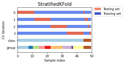
- StratifiedKFold
- RepeatedStratifiedKFold
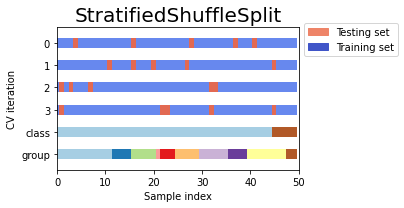
- StratifiedShuffleSplit
Note: Folds obtained via StratifiedShuffleSplit may not be completely different.
LogisticRegressionCV
- Support in-build cross validation for optimizing hyperparameters
- The following are key parameters for HPT and cross validation
cv specifies cross validation iterator
scoring specifies scoring function to use for HPT
cs specifies regularization strengths to experiment with.
- Choosing the best hyper-parameters
refit = True
refit = False
Scores averaged across folds, values corresponding to the best score are selected and final refit with these parameters
the coefs, intercepts and C that correspond to the best scores across folds are averaged.
Now let's look at classification metrics implemented in sklearn.
sklearn.metrics implements a bunch of classification scoring metrics based on true labels and predicted labels as inputs.
accuracy_score
balanced_accuracy_score
top_k_accuracy_score
roc_auc_score
precision_score
recall_score
f1_score
score(actual_labels, predicted_labels)
Classification metrics
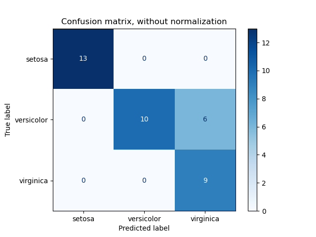
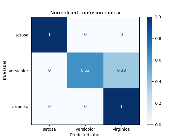
Confusion matrix
-
confusion_matrixevaluates classification accuracy by computing the confusion matrix with each row corresponding to the true class.
from sklearn.metrics import confusion_matrix
confusion_matrix(y_true, y_predicted)
Entry \(i,j\) in a confusion matrix
Example:
number of observations actually in group \(i\), but predicted to be in group \(j\).
Confusion matrix can be displayed with ConfusionMatrixDisplay API in sklearn.metrics.
- Confusion matrix
- From estimators
- From predictions
ConfusionMatrixDisplay(confusion_matrix=cm, display_labels=clf.classes_)ConfusionMatrixDisplay.from_estimator(clf, X_test, y_test)ConfusionMatrixDisplay.from_predictions(y_test, y_pred)The classification_report function builds a text report showing the main classification metrics.
from sklearn.metrics import classification_report
print(classification_report(y_true, y_predicted))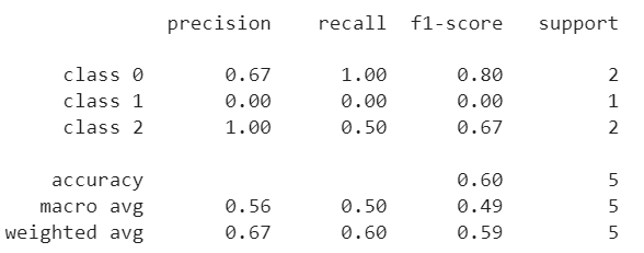
Classifier Performance across probability thresholds
from sklearn.metrics import precision_recall_curve
precision, recall, thresholds = precision_recall_curve(y_true, y_predicted)
from sklearn.metrics import roc_curve
fpr, tpr, thresholds = metrics.roc_curve(y_true, y_scores, pos_label=2)How to extend binary metric to multiclass or multilabel problems?
- Treat data as a collection of binary problems, one for each class.
- Then, average binary metric calculations across the set of classes.
-
Can be done using
averageparameter.
calculates the mean of the binary metrics
computes the average of binary metrics in which each class’s score is weighted by its presence in the true data sample.
gives each sample-class pair an equal contribution to the overall metric
calculates the metric over the true and predicted classes for each sample in the evaluation data, and returns their average
returns an array with the score for each class
macro
weighted
micro
samples
None
Summary
- Classification specific cross validation iterator based on stratification.
- Classification metrics
- Extending binary metrics to multi-learning set up.
Naive Bayes Classifier
- Naive Bayes classifier applies Bayes’ theorem with the “naive” assumption of conditional independence between every pair of features given the value of the class variable.
Naive Bayes classifier
For a given class variable \(y\) and dependent feature vector \(x_1\) through \(x_m\),
the naive conditional independence assumption is given by:
Naive Bayes learners and classifiers can be extremely fast compared to more sophisticated methods.
List of NB Classifiers
ComplementNB
GaussianNB
BernoulliNB
CategoricalNB
MultinomialNB
- Implemented in sklearn.naive_bayes module
- Implements fit method to estimate parameters of NB classifier with feature matrix and labels as inputs.
- The prediction is performed using predict method.
Which NB to use if data is only numerical?
GaussianNB
implements the Gaussian Naive Bayes algorithm for classification
from sklearn.naive_bayes import GaussianNB
gnb = GaussianNB()
gnb.fit(X_train, y_train)
Instantiate a GaussianNBClassifer estimator and then call fit method using X_train and y_train.
Which NB to use if data is multinomially distributed?
MultinomialNB
implements the naive Bayes algorithm for multinomially distributed data
(text classification)
from sklearn.naive_bayes import MultinomialNB
mnb = MultinomialNB()
mnb.fit(X_train, y_train)
Instantiate a MultinomialNBClassifer estimator and then call fit method using X_train and y_train.
What to do if data is imbalanced ?
ComplementNB
implements the complement naive Bayes (CNB) algorithm.
from sklearn.naive_bayes import ComplementNB
cnb = ComplementNB()
cnb.fit(X_train, y_train)
Instantiate a ComplementNBClassifer estimator and then call fit method using X_train and y_train.
CNB regularly outperforms MNB (often by a considerable margin) on text classification tasks.
What to do if data has multivariate Bernoulli distributions?
BernoulliNB
- implements the naive Bayes algorithm for data that is distributed according to multivariate Bernoulli distributions
from sklearn.naive_bayes import BernoulliNB
bnb = BernoulliNB()
bnb.fit(X_train, y_train)
Instantiate a BernoulliNBClassifer estimator and then call fit method using X_train and y_train.
- each feature is assumed to be a binary-valued (Bernoulli, boolean) variable
What to do if data is categorical ?
CategoricalNB
implements the categorical naive Bayes algorithm suitable for classification with discrete features that are categorically distributed
from sklearn.naive_bayes import CategoricalNB
canb = CategoricalNB()
canb.fit(X_train, y_train)
Instantiate a CategoricalNBClassifer estimator and then call fit method using X_train and y_train.
assumes that each feature, which is described by the index \(i\), has its own categorical distribution.
Week #7
-
It is a type of instance-based learning or non-generalizing learning
- does not attempt to construct a model
- simply stores instances of the training data
Nearest neighbor classifier
- Classification is computed from a simple majority vote of the nearest neighbors of each point.
- Two different implementations of nearest neighbors classifiers are available.
- KNeighborsClassifier
- RadiusNeighborsClassifier
How are KNeighborsClassifier and RadiusNeighborsClassifier different?
KNeighborsClassifier
RadiusNeighborsClassifier
- learning based on the k nearest neighbors
- learning based on the number of neighbors within a fixed radius r of each training point
- most commonly used technique
- used in cases where the data is not uniformly sampled
- choice of the value k is highly data-dependent
- fixed value of r is specified, such that points in sparser neighborhoods use fewer nearest neighbors for the classification
How do you apply KNeighborsClassifier?
Step 1: Instantiate a KNeighborsClassifer estimator without passing any arguments to it to create a classifer object.
from sklearn.neighbors import KNeighborsClassifier
kneighbor_classifier = KNeighborsClassifier()
Step 2: Call fit method on KNeighbors classifier object with training feature matrix and label vector as arguments.
# Model training with feature matrix X_train and
# label vector or matrix y_train
kneighbor_classifier.fit(X_train, y_train)
How do you specify the number of nearest neighbors in KNeighborsClassifier?
-
Specify the number of nearest neighbors K from the training dataset using
n_neighborsparameter.- value should be int.
kneighbor_classifier = KNeighborsClassifier(n_neighbors = 3)What is the default value of K?
n_neighbors = 5
How do you assign weights to neighborhood in KNeighborsClassifier?
- It is better to weight the neighbors such that nearer neighbors contribute more to the fit.
weights
- ‘uniform’ : All points in each neighborhood are weighted equally.
- ‘distance’ : weight points by the inverse of their distance.
- closer neighbors of a query point will have a greater influence than neighbors which are further away.
kneighbor_classifier = KNeighborsClassifier(weights= 'uniform')Default:
Can we define our own weight values for KNeighborsClassifier?
- Yes, it is possible if you have an array of distances.
weightsparameter also accepts a user-defined function which takes an array of distances as input, and returns an array of the same shape containing the weights.
def user_weights(weights_array):
    return weights_array

kneighbor_classifier = KNeighborsClassifier(weights=user_weights)
Example:
Which algorithm is used to compute the nearest neighbors in KNeighborsClassifier?
algorithm
‘ball_tree’ will use BallTree
‘kd_tree’ will use KDTree
‘brute’ will use a brute-force search
‘auto’ will attempt to decide the most appropriate algorithm based on the values passed to the fit method.
kneighbor_classifier = KNeighborsClassifier(algorithm='auto')Default:
Some additional parmeters for tree algorithm in KNeighborsClassifier?
leaf_size
For 'ball_tree' and 'kd_tree' algorithms, there are some other parameters to be set.
metric
p
- can affect the speed of the construction and query, as well as the memory required to store the tree
- default = 30
- Distance metric to use for the tree
-
It is either string or callable function
-
some metrics are listed below:
- “euclidean”, “manhattan”, “chebyshev”, “minkowski”, “wminkowski”, “seuclidean”, “mahalanobis”
-
some metrics are listed below:
- default = 'minkowski'
- Power parameter for the Minkowski metric.
- default = 2
How do you apply RadiusNeighborsClassifier?
Step 1: Instantiate a RadiusNeighborsClassifer estimator without passing any arguments to it to create a classifer object.
from sklearn.neighbors import RadiusNeighborsClassifier
radius_classifier = RadiusNeighborsClassifier()
Step 2: Call fit method on RadiusNeighbors classifier object with training feature matrix and label vector as arguments.
# Model training with feature matrix X_train and
# label vector or matrix y_train
radius_classifier.fit(X_train, y_train)
How do you specify the number of neighbors in RadiusNeighborsClassifier?
-
The number of neighbors is specified within a fixed radius r of each training point using
radiusparameter. - r is a float value.
radius_classifier = RadiusNeighborsClassifier(radius=1.0)What is the default value of r ?
r = 1.0
Parameters for RadiusNeighborsClassifier
weights
algorithm
‘uniform’
‘distance’
[callable] function
default = 'uniform'
‘ball_tree’
‘kd_tree’
‘brute’
default = ‘auto’
‘auto’
leaf_size
metric
p
default = 30
default = 'minkowski'
default = 2
Appendix
We shall discuss two modules:
Multiclass and multilabel classification
Multiclass classification
(sklearn.multiclass)
Multilabel classification
(sklearn.multioutput)
problem types
meta-estimators
OneVsOneClassifier
OneVsRestClassifier
OutputCodeClassifier
MultiOutputClassifier
ClassifierChain
- Multiclass classification is a classification task with more than two classes. Each sample can only be labeled as one class.
-
Multilabel classification is a classification task labeling each sample with m labels from
n_classespossible classes.
How to determine the type of data indicated by the target for multiclass and multilabel classification?
from sklearn.utils.multiclass import type_of_target
type_of_target(y)- Within scikit-learn, all estimators supporting binary classification also support multiclass classification, using One-vs-Rest by default.
- A target may be represented in different forms for classification problems.
Input paramter : y (array-like)
Output : target_type (string)
type_of_target(y)
Multilabel classification
OneVsRestClassifier
OneVsOneClassifier
OutputCodeClassifier
- Fitting one classifier per class.
- For each classifier, the class is fitted against all the other classes.
-
Constructs one classifier per pair of classes.
-
At prediction time, the class which received the most votes is selected.
- Each class is represented in a Euclidean space, where each dimension can only be 0 or 1 (binary code)
Example for OneVsRestClassifier
from sklearn import datasets
from sklearn.multiclass import OneVsRestClassifier
from sklearn.linear_model import SGDClassifier
from sklearn.model_selection import train_test_split

X, y = datasets.load_iris(return_X_y=True)
X_train, X_test, y_train, y_test = train_test_split(X,y,test_size=0.3)
clf = OneVsRestClassifier(SGDClassifier(loss = 'hinge'))
clf = clf.fit(X_train, y_train)
y_pred = clf.predict(X_test)
print('y_test',y_test)
print('y_pred',y_pred)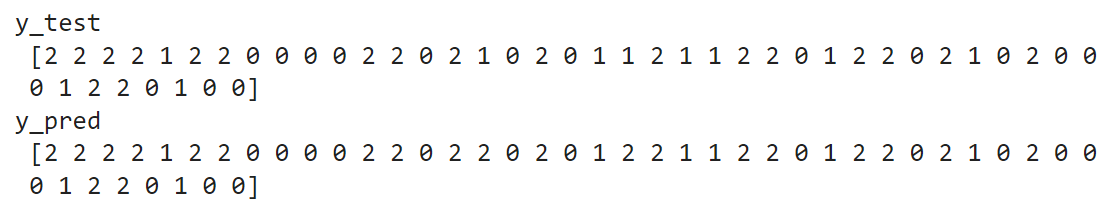
We shall use iris dataset which contains 150 datapoints each with 4 features and 3 labels.
Example for OneVsOneClassifier
from sklearn import datasets
from sklearn.multiclass import OneVsOneClassifier
from sklearn.linear_model import SGDClassifier
from sklearn.model_selection import train_test_split

X, y = datasets.load_iris(return_X_y=True)
X_train, X_test, y_train, y_test = train_test_split(X,y,test_size=0.3)
clf = OneVsOneClassifier(SGDClassifier(loss = 'hinge'))
clf = clf.fit(X_train, y_train)
y_pred = clf.predict(X_test)
print('y_test',y_test)
print('y_pred',y_pred)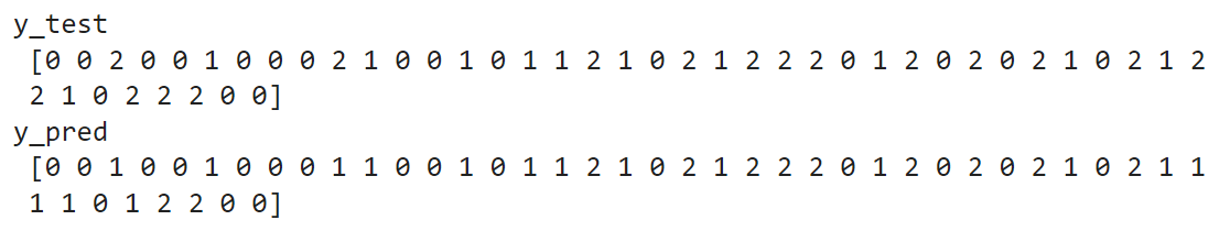
Example for MultiOutputClassifier
import numpy as np
from sklearn.datasets import make_multilabel_classification
from sklearn.utils.multiclass import type_of_target
from sklearn.multioutput import MultiOutputClassifier
from sklearn.neighbors import KNeighborsClassifier

X, y = make_multilabel_classification(n_classes=3, random_state=0)
print('target is a', type_of_target(y))
clf = MultiOutputClassifier(KNeighborsClassifier(n_neighbors=2))
clf = clf.fit(X, y)
y_test = y[-2:]
y_pred = clf.predict(X[-2:])
print('y_test \n',y_test)
print('y_pred \n',y_pred)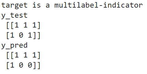
We shall create a synthetic multilabel dataset for this example.
Example for ClassiferChainClassifier
import numpy as np
import matplotlib.pyplot as plt
from sklearn.datasets import fetch_openml
from sklearn.multioutput import ClassifierChain
from sklearn.model_selection import train_test_split
from sklearn.multiclass import OneVsRestClassifier
from sklearn.metrics import jaccard_score
from sklearn.linear_model import LogisticRegression

# Load a multi-label dataset
X, Y = fetch_openml("yeast", version=4, return_X_y=True)
Y = Y == "TRUE"
X_train, X_test, Y_train, Y_test = train_test_split(X, Y, test_size=0.2, random_state=0)

base_lr = LogisticRegression()
ovr = OneVsRestClassifier(base_lr)
ovr.fit(X_train, Y_train)- We shall use yeast dataset which contains 2417 datapoints each with 103 features and 14 possible labels.
- Let us fit an independent logistic regression model for each class using the OneVsRestClassifier wrapper.
Example for ClassiferChain
Y_pred_ovr = ovr.predict(X_test)
ovr_jaccard_score = jaccard_score(Y_test, Y_pred_ovr, average="samples")
chains = [ClassifierChain(base_lr, order="random", random_state=i) for i in range(4)]
for chain in chains:
    chain.fit(X_train, Y_train)
Y_pred_chains = np.array([chain.predict(X_test) for chain in chains])
Y_pred_chains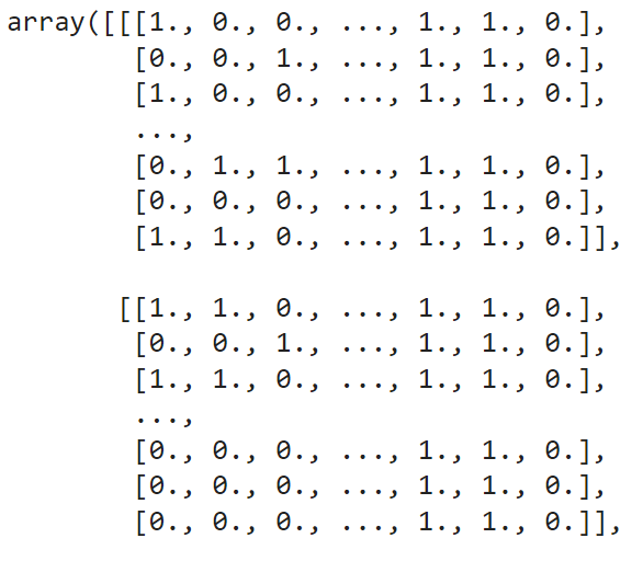
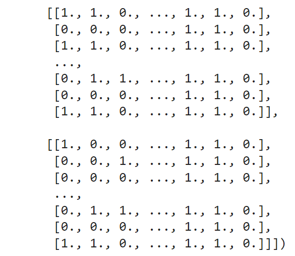
Example for ClassiferChain
chain_jaccard_scores = [
jaccard_score(Y_test, Y_pred_chain >= 0.5, average="samples")
for Y_pred_chain in Y_pred_chains]
Y_pred_ensemble = Y_pred_chains.mean(axis=0)
ensemble_jaccard_score = jaccard_score(Y_test, Y_pred_ensemble >= 0.5, average="samples")
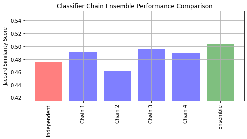
model_scores = [ovr_jaccard_score] + chain_jaccard_scores
model_scores.append(ensemble_jaccard_score)
model_names = ("Independent","Chain 1","Chain 2","Chain 3","Chain 4","Ensemble")
# Let us plot all the scores
x_pos = np.arange(len(model_names))
fig, ax = plt.subplots(figsize=(7, 4))
ax.grid(True)
ax.set_title("Classifier Chain Ensemble Performance Comparison")
ax.set_xticks(x_pos)
ax.set_xticklabels(model_names, rotation="vertical")
ax.set_ylabel("Jaccard Similarity Score")
ax.set_ylim([min(model_scores) * 0.9, max(model_scores) * 1.1])
colors = ["r"] + ["b"] * len(chain_jaccard_scores) + ["g"]
ax.bar(x_pos, model_scores, alpha=0.5, color=colors)
plt.tight_layout()
plt.show()- Let us fit an ensemble of logistic regression classifier chains and take the average prediction of all the chains.
Output of ClassifierChain
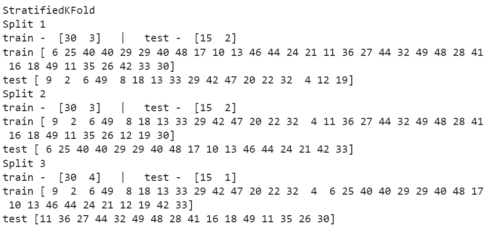
from sklearn.model_selection import StratifiedKFold, StratifiedShuffleSplit
import numpy as np
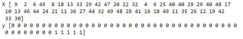
X, y = np.random.randint(1,50,50), np.hstack(([0] * 45, [1] * 5))
print('X',X)
print('y',y)
skf = StratifiedKFold(n_splits=3)
print('StratifiedKFold')
count = 1
for train, test in skf.split(X, y):
print('Split', count)
print('train - {} | test - {}'.format(np.bincount(y[train]), np.bincount(y[test])))
print('train',X[train])
print('test',X[test])
count+=1
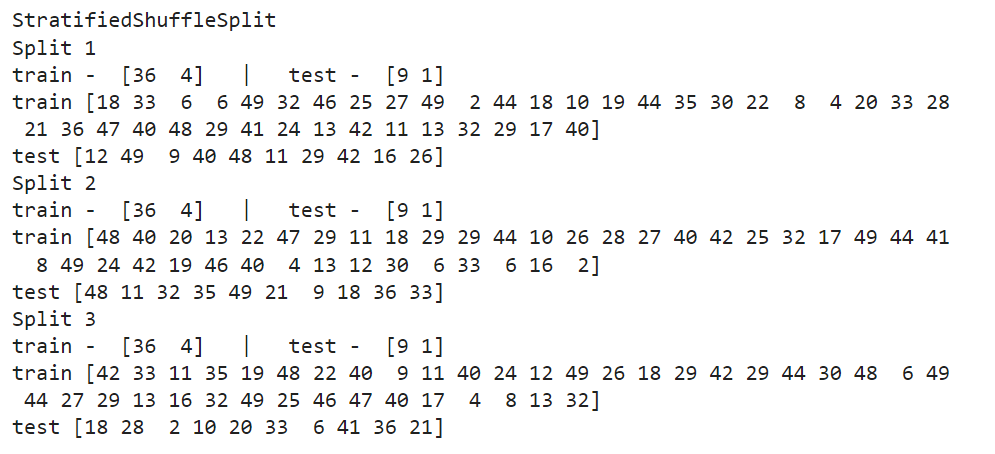
print('StratifiedShuffleSplit')
sss = StratifiedShuffleSplit(n_splits=3, test_size=0.2, random_state=0)
count = 1
for train_index, test_index in sss.split(X, y):
print('Split', count)
print('train - {} | test - {}'.format(np.bincount(y[train_index]), np.bincount(y[test_index])))
print('train',X[train_index])
print('test',X[test_index])
count+=1Example to compare StratifiedKFold and StratifiedShuffleSplit
Output:
Comparison
- The calibration module allows you to better calibrate the probabilities of a given model, or to add support for probability prediction.
- obtain a probability of the respective label
Probability calibration
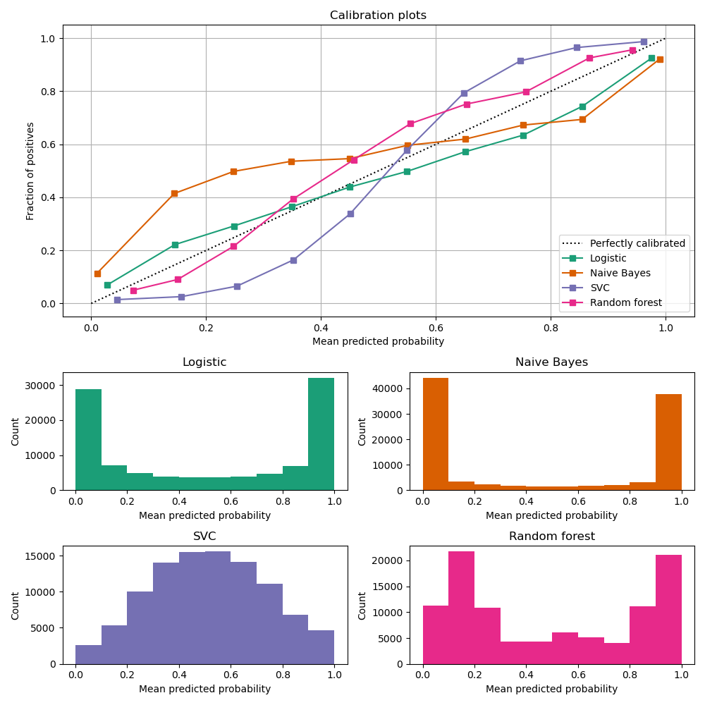
Calibration curves
compare how well the probabilistic predictions of a binary classifier are calibrated.
plots the true frequency of the positive label against its predicted probability, for binned predictions.
x axis : average predicted probability in each bin
y axis : fraction of positives, i.e. the proportion of samples whose class is the positive class (in each bin).
Probability calibration - Example

Image Source: https://scikit-learn.org/stable/modules/calibration.html
- Calibration curve plot is created with CalibrationDisplay.from_estimators, which uses calibration_curve to calculate the per bin average predicted probabilities and fraction of positives.
Probability calibration - Example
LogisticRegression returns well calibrated predictions by default as it directly optimizes Log loss.
GaussianNB tends to push probabilities to 0 or 1.
RandomForestClassifier peaks at approximately 0.2 and 0.9 probability, while probabilities close to 0 or 1 are very rare.
LinearSVC focus on difficult to classify samples that are close to the decision boundary (the support vectors).
- Fitting a regressor (called a calibrator) that maps the output of the classifier to a calibrated probability in [0, 1].
How to calibrate a classifier?
from sklearn.metrics from sklearn.calibration import CalibratedClassifierCV
calibrated_clf = CalibratedClassifierCV()
estimates the parameters of a classifier and subsequently calibrates a classifier
CalibratedClassifierCV
Some parameters for CalibratedClassifierCV
base_estimator
method
ensemble
- Can be ‘sigmoid’ which corresponds to Platt’s method (i.e. a logistic regression model) or ‘isotonic’ which is a non-parametric approach
- default = 'sigmoid'
-
determines how the calibrator is fitted when
cvis not'prefit'. -
ignored if
cv='prefit'. - default = True
cv
- determines the cross-validation splitting strategy
- default = None
- classifier whose output needs to be calibrated
- default = None
Appendix
- Ridge classification
- Logistic regression
- SGD classifier
- Perceptron
- Extending linear models with polynomial features
- Nearest neighbor classifier
- NB classifier
- Multi-label and multi-class classification
- Probability calibration
- Model selection for classification
- CV
- HPT
- Classification metrics
Contents
Class: sklearn.linear_model.RidgeClassifier
Some Parameters:
- alpha - Regularization strength; must be a positive float (default = 1.0).
-
solver - used in the computational routines: (default = 'auto')
- ‘auto’ - chooses the solver automatically based on the type of data
- ‘svd’ - uses Singular Valur Decomposition
- ‘cholesky’ - uses scipy.linalg.solve function to obtain a closed-form solution
- ‘lsqr’ - uses the dedicated regularized least-squares routine scipy.sparse.linalg.lsqr. (fastest and uses an iterative procedure)
- ‘sparse_cg’ - uses the conjugate gradient solver of scipy.sparse.linalg.cg.
- 'sag’ - uses a Stochastic Average Gradient descent iterstive procedure
- ‘saga’ - unbiased and more flexible version of 'sag'
Ridge classification
Class: sklearn.linear_model.LogisticRegression
Some Parameters:
-
penalty (default = 'l2')
-
'none' - no penalty is added
-
'l2' - add a L2 penalty term and it is the default choice
-
'l1' - add a L1 penalty term
-
'elasticnet' - both L1 and L2 penalty terms are added
-
-
solver (default = 'lbfgs')
-
'liblinear' - uses a coordinate descent (CD) algorithm
-
'lbfgs' - an optimizer in the family of quasi-Newton methods.
-
'newton-cg', 'sag', 'saga'
-
Logistic regression
- For small datasets, ‘liblinear’ is a good choice, whereas ‘sag’ and ‘saga’ are faster for large ones.
- For multiclass problems, only ‘newton-cg’, ‘sag’, ‘saga’ and ‘lbfgs’ handle multinomial loss.
- ‘liblinear’ is limited to one-versus-rest schemes.
-
max_iter (default = 100)
- maximum number of iterations taken for the solvers to converge
-
multi_class (default = ‘auto’)
- ‘ovr’ - a binary problem is fit for each label (uses the one-vs-rest)
- ‘multinomial’ - uses the cross-entropy loss
- ‘auto’ - selects ‘ovr’ if the data is binary, or if solver=’liblinear’, and otherwise selects ‘multinomial’.
Logistic regression
- Stochastic Gradient Descent (SGD) is a simple yet very efficient approach to fitting linear classifiers and regressors under convex loss functions
- It is an optimization technique and does not correspond to a specific family of machine learning models.
- It is only a way to train a model.
- easily scale to problems with more than \(10^5\) training examples and more than \(10^5\) features
-
SGD has to be fitted with two arrays:
- training samples - X, an array of shape (n_samples, n_features)
- target values (class labels) - y, an array of shape (n_samples,)
SGDClassifier(loss='log')
LogisticRegression(solver='sgd')
SGD classifier
SGDClassifier(loss='hinge')
Linear Support vector machine
SGD classifier
-
Class:
sklearn.linear_model.SGDClassifier-
This estimator implements regularized linear models with SGD.
-
The gradient of the loss is estimated each sample at a time and the model is updated along the way with a decreasing learning rate.
-
-
Some parameters
-
penalty - 'l2’, ‘l1’, ‘elasticnet’ (default = 'l2')
-
loss (default = 'hinge')
-
'hinge' - (soft-margin) linear Support Vector Machine,
-
'modified_huber' - smoothed hinge loss brings tolerance to outliers as well as probability estimates
-
'log' - logistic regression
-
'squared_hinge' - like hinge but is quadratically penalized
-
'perceptron' - linear loss used by the perceptron algorithm
-
regression losses - ‘squared_error’, ‘huber’, ‘epsilon_insensitive’, or ‘squared_epsilon_insensitive’
-
-
SGD classifier
-
alpha (default = 0.0001)
-
constant that multiplies the regularization term.
-
-
fit_intercept (default = True)
-
If False, the data is assumed to be already centered.
-
-
max_iter (default = 1000)
-
maximum number of passes over the training data (aka epochs).
-
-
learning_rate (default = ’optimal’)
-
‘constant’:
eta = eta0(default eta0=0.0, initial learning rate) -
‘optimal’:
eta = 1.0 / (alpha * (t + t0))where t0 is chosen by a heuristic proposed by Leon Bottou. -
‘invscaling’:
eta = eta0 / pow(t, power_t) -
‘adaptive’:
eta = eta0, as long as the training keeps decreasing. Each time n_iter_no_change consecutive epochs fail to decrease the training loss by tol or fail to increase validation score by tol if early_stopping is True, the current learning rate is divided by 5.
-
SGD classifier
-
tol (default = 1e-3)
-
stopping criterion.
-
If it is not None, training will stop when (loss > best_loss - tol) for
n_iter_no_changeconsecutive epochs. -
Convergence is checked against the training loss or the validation loss depending on the
early_stoppingparameter.
-
-
early_stopping (default = False)
-
to terminate training when validation score is not improving.
-
If set to True, it will automatically set aside a stratified fraction of training data as validation and terminate training when validation score returned by the
scoremethod is not improving by at least tol for n_iter_no_change consecutive epochs
-
SGD classifier
-
validation_fraction (default = 0.1)
-
proportion of training data to set aside as validation set for
early stopping. Must be between 0 and 1. -
Only used if
early_stopping
-
-
n_iter_no_change (default = 5)
-
Number of iterations with no improvement to wait before stopping fitting.
-
Convergence is checked against the training loss or the validation loss depending on the
early_stopping
-
-
class_weight (default = None) {class_label: weight} or “balanced”,
-
The “balanced” mode uses the values of y to automatically adjust weights inversely proportional to class frequencies in the input data as
n_samples / (n_classes * np.bincount(y)). -
Preset for the class_weight fit parameter. Weights associated with classes. If not given, all classes are supposed to have weight one.
-
It is a simple classification algorithm suitable for large-scale learning.
Class: sklearn.linear_model.Perceptron
Some Parameters:
-
penalty - 'l2’, ‘l1’, ‘elasticnet’ (default = 'l2')
-
alpha - (default = 0.0001)
-
l1_ratio - (default = 0.15)
-
fit_intercept - (default = True)
-
max_iter - (default = 1000)
-
tol - (default = 1e-3)
-
eta0 - (default = 1)
-
early_stopping - (default = False)
-
validation_fraction - (default = 0.1)
-
n_iter_no_change - (default = 5)
-
Type of instance-based learning or non-generalizing learning
- it does not attempt to construct a general internal model, but simply stores instances of the training data.
- Classification is computed from a simple majority vote of the nearest neighbors of each point.
scikit-learnimplements two different nearest neighbors classifiers.
Nearest neighbor classifier
| KNeighborsClassifier | RadiusNeighborsClassifier |
|---|---|
| implements learning based on the k nearest neighbors of each query point, where k is an integer value specified by the user. | implements learning based on the number of neighbors within a fixed radius r of each training point, where r is a floating-point value specified by the user. |
| most commonly used technique choice of the value k is highly data-dependent |
used in cases where the data is not uniformly sampled |
| larger k suppresses the effects of noise, but makes the classification boundaries less distinct. | user specifies a fixed radius r, such that points in sparser neighborhoods use fewer nearest neighbors for the classification |
Class: sklearn.neighbors.KNeighborsClassifier
Some Parameters
-
n_neighbors (default = 5)
- Number of neighbors to use by default for k neighbors queries.
-
weights (used in prediction) (default = ’uniform')
- ‘uniform’ : All points in each neighborhood are weighted equally.
- ‘distance’ : weight points by the inverse of their distance. in this case, closer neighbors of a query point will have a greater influence than neighbors which are further away.
- [callable] : a user-defined function which accepts an array of distances, and returns an array of the same shape containing the weights.
Nearest neighbor classifier
- algorithm (default = 'auto')
-
leaf_size (default = 30)
- Leaf size passed to BallTree or KDTree.
-
p (default = 2)
- Power parameter for the Minkowski metric.
- When p = 1, this is equivalent to using manhattan_distance (l1), and euclidean_distance (l2) for p = 2.
- For arbitrary p, minkowski_distance (l_p) is used.
Nearest neighbor classifier
Class: sklearn.neighbors.RadiusNeighborsClassifier
Some Parameters
-
radius (default = 1.0)
-
Range of parameter space to use by default for radius_neighbors queries
-
-
weights (‘uniform’, ‘distance’, [callable], default = ’uniform')
-
algorithm (‘ball_tree’, ‘kd_tree’, ‘brute’, ‘auto’, default = 'auto'
-
leaf_size (default = 30)
-
p (default = 2)
-
metric (default = ’minkowski’)
-
Distance metric to use for the tree.
-
Nearest neighbor classifier
- Naive Bayes methods are a set of supervised learning algorithms based on applying Bayes’ theorem with the “naive” assumption of conditional independence between every pair of features given the value of the class variable.
Naive Bayes classification
GaussianNB
MultinomialNB
ComplementNB
CategoricalNB
BernoulliNB
implements the Gaussian Naive Bayes algorithm for classification
implements the naive Bayes algorithm for multinomially distributed data (text classification)
implements the complement naive Bayes (CNB) algorithm. (suited for imbalanced data sets)
implements the naive Bayes training and classification algorithms for data that is distributed according to multivariate Bernoulli distributions
implements the categorical naive Bayes algorithm for categorically distributed data.
- We shall discuss two modules: sklearn.multiclass and sklearn.multioutput.
- Multiclass classification is a classification task with more than two classes. Each sample can only be labeled as one class.
- Multilabel classification is a classification task labeling each sample with m labels from n_classes possible classes.
Multiclass and multilabel classification
Multiclass classification
(sklearn.multiclass)
Multilabel classification
(sklearn.multioutput)
problem types
meta-estimators
OneVsOneClassifier
OneVsRestClassifier
OutputCodeClassifier
MultiOutputClassifier
ClassifierChain
sklearn.utils.multiclass.type_of_target
-
determines the type of data indicated by the target.
-
Parameters : y (array-like), Returns : target_type (string)
Multiclass classification - Target format
| target_type | y |
|---|---|
| 'continuous' | array-like of floats that are not all integers and is 1d or a column vector. |
| 'continuous-multioutput' | 2d array of floats that are not all integers, and both dimensions are of size > 1. |
| ‘binary’ | contains <= 2 discrete values and is 1d or a column vector. |
| ‘multiclass’ | contains more than two discrete values, is not a sequence of sequences, and is 1d or a column vector. |
| ‘multiclass-multioutput’ | 2d array that contains more than two discrete values, is not a sequence of sequences, and both dimensions are of size > 1. |
| ‘unknown’ | array-like but none of the above, such as a 3d array, sequence of sequences, or an array of non-sequence objects. |
Examples
>>> from sklearn.utils.multiclass import type_of_target
>>> import numpy as np
>>> type_of_target([0.1, 0.6])
'continuous'
>>> type_of_target([1, -1, -1, 1])
'binary'
>>> type_of_target(['a', 'b', 'a'])
'binary'
>>> type_of_target([1.0, 2.0])
'binary'>>> type_of_target([1, 0, 2])
'multiclass'
>>> type_of_target([1.0, 0.0, 3.0])
'multiclass'
>>> type_of_target(['a', 'b', 'c'])
'multiclass'>>> type_of_target(np.array([[1, 2], [3, 1]]))
'multiclass-multioutput'>>> type_of_target(np.array([[1.5, 2.0], [3.0, 1.6]]))
'continuous-multioutput'continuous-multioutput
continuous
binary
multiclass
multiclass-multioutput
-
OneVsRestClassifier
- Fitting one classifier per class. For each classifier, the class is fitted against all the other classes.
- classifiers needed = \(n_{classes}\)
- advantage : interpretability.
- most commonly used strategy and is a fair default choice.
-
-
Constructs one classifier per pair of classes.
-
At prediction time, the class which received the most votes is selected. In the event of a tie, it selects the class with the highest aggregate classification confidence by summing over the pair-wise classification confidence levels computed by the underlying binary classifiers.
-
classifiers needed = \(\dfrac{n_{classes}\times(n_{classes} - 1)}{2} \)
-
slower than one-vs-the-rest, due to its \(O(n_{classes}^2)\) complexity.
-
advantage : for kernel algorithms which don’t scale well
-
Multiclass classification
-
OutputCodeClassifier
-
Error-Correcting Output Code-based strategy
- each class is represented in a Euclidean space, where each dimension can only be 0 or 1 (binary code)
- the code_size attribute allows the user to control the number of classifiers which will be used. It is a percentage of the total number of classes.
-
Error-Correcting Output Code-based strategy
Multiclass classification
Multilabel classification - Target format
| target_type | y |
|---|---|
| ‘multilabel-indicator’ | label indicator matrix, an array of two dimensions with at least two columns, and at most 2 unique values. |
type_of_target(np.array([[0, 1], [1, 1]]))
'multilabel-indicator'
>>> type_of_target([[1, 2]])
'multilabel-indicator'
multilabel-indicator
Example for OutputCodeClassifier
from sklearn import datasets
from sklearn.multiclass import OutputCodeClassifier
from sklearn.linear_model import SGDClassifier
from sklearn.model_selection import train_test_split

X, y = datasets.load_iris(return_X_y=True)
X_train, X_test, y_train, y_test = train_test_split(X,y,test_size=0.3)
clf = OutputCodeClassifier(SGDClassifier(loss = 'hinge'),code_size=2,)
clf = clf.fit(X_train, y_train)
y_pred = clf.predict(X_test)
print('y_test',y_test)
print('y_pred',y_pred)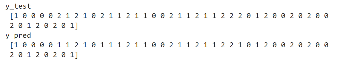
Multilabel classification
| MultiOutputClassifier | ClassifierChain |
|---|---|
| Strategy consists of fitting one classifier per target. | Way of combining a number of binary classifiers into a single multi-label model that is capable of exploiting correlations among targets. |
| Allows multiple target variable classifications. Able to estimate a series of target functions that are trained on a single predictor matrix to predict a series of responses. |
For a multi-label classification problem with N classes, N binary classifiers are assigned an integer between 0 and N-1. These integers define the order of models in the chain. |
- The calibration module allows you to better calibrate the probabilities of a given model, or to add support for probability prediction.
- obtain a probability of the respective label
Probability calibration
Calibration curves
compare how well the probabilistic predictions of a binary classifier are calibrated.
plots the true frequency of the positive label against its predicted probability, for binned predictions.
x axis : average predicted probability in each bin
y axis : fraction of positives, i.e. the proportion of samples whose class is the positive class (in each bin).
Probability calibration - Example
Image Source: https://scikit-learn.org/stable/modules/calibration.html
- Calibration curve plot is created with CalibrationDisplay.from_estimators, which uses calibration_curve to calculate the per bin average predicted probabilities and fraction of positives.
Probability calibration - Example
LogisticRegression returns well calibrated predictions by default as it directly optimizes Log loss.
GaussianNB tends to push probabilities to 0 or 1.
RandomForestClassifier peaks at approximately 0.2 and 0.9 probability, while probabilities close to 0 or 1 are very rare.
LinearSVC focus on difficult to classify samples that are close to the decision boundary (the support vectors).
- Fitting a regressor (called a calibrator) that maps the output of the classifier (as given by decision_function or predict_proba) to a calibrated probability in [0, 1].
-
CalibratedClassifierCV class is used to calibrate a classifier.
- estimates the parameters of a classifier and subsequently calibrates a classifier.
-
ensemble = True- for each cv split it fits a copy of the base estimator to the training subset, and calibrates it using the testing subset.
- For prediction, predicted probabilities are averaged across these individual calibrated classifiers.
-
ensemble = False- cv is used to obtain unbiased predictions, which are then used for calibration.
- For prediction, the base estimator, trained using all the data, is used.
Calibrating a classifier
-
Cross-validation iterators with stratification based on class labels:
- There is a chance for a large imbalance in the distribution of the target classes for some classification problems.
- Recommendation:
- These two methods ensure that, in each train and validation fold, relative class frequencies are approximately preserved.
-
Cross-validation estimator:
- Cross-validation estimators are named EstimatorCV and tend to be roughly equivalent to GridSearchCV(Estimator(), ...).
- Example of cross-validation estimator is LogisticRegressionCV.
Model selection for classification
- This cross-validation object returns stratified folds by preserving the percentage of samples for each class.
Class: sklearn.model_selection.StratifiedKFold
Some Parameters:
-
n_splits (default = 5)
-
Number of folds. Must be at least 2.
-
-
shuffle (default = False)
-
to shuffle or not to shuffle each class’s samples before splitting into batches.
-
samples within each split will not be shuffled.
-
-
random_state RandomState instance or None, (default=None)
-
set
random_statewhenshuffle = Truebecause it affects the ordering of the indices, which controls the randomness of each fold for each class.
-
- RepeatedStratifiedKFold: Repeats Stratified K-Fold n times.
1. Stratified k-fold
- Splits preserve the same percentage for each target class as in the complete set but do not guarantee that all folds will be different.
Class: sklearn.model_selection.StratifiedShuffleSplit
Some Parameters:
- n_splits (default = 10)
- random_state (RandomState instance or None, default = None)
-
test_size (default = None)
- float value - proportion of the test dataset split (between 0.0 and 1.0)
- int value - represents the absolute number of test samples
- None - complement of the train size. If train_size = None, value = 0.1
-
train_size (default = None)
- float value - proportion of the train dataset split (between 0.0 and 1.0)
- int value - absolute number of train samples.
- None - complement of the test size.
2. StratifiedShuffleSplit
from sklearn.model_selection import StratifiedKFold, StratifiedShuffleSplit
import numpy as np
X, y = np.random.randint(1,50,50), np.hstack(([0] * 45, [1] * 5))
print('X',X)
print('y',y)
skf = StratifiedKFold(n_splits=3)
print('StratifiedKFold')
count = 1
for train, test in skf.split(X, y):
  print('Split', count)
  print('train -  {}   |   test -  {}'.format(np.bincount(y[train]), np.bincount(y[test])))
  print('train',X[train])
  print('test',X[test])
  count+=1
print('StratifiedShuffleSplit')
sss = StratifiedShuffleSplit(n_splits=3, test_size=0.2, random_state=0)
count = 1
for train_index, test_index in sss.split(X, y):
  print('Split', count)
  print('train -  {}   |   test -  {}'.format(np.bincount(y[train_index]), np.bincount(y[test_index])))
  print('train',X[train_index])
  print('test',X[test_index])
  count+=1
Example to compare StratifiedKFold and StratifiedShuffleSplit
Output:
Comparison
3. Logistic Regression CV
- Logistic regression with tuning the hyperparameter
Csvalues andl1_ratiosvalues.
Class: sklearn.linear_model.LogisticRegressionCV
Some Parameters:
-
'Cs' (default = 10)
-
Each of the values in Cs describes the inverse of regularization strength.
-
If int, then a grid of values = logarithmic scale between \(1e^{-4}\) & \(1e^4\).
-
-
'cv' (default = None)
-
The default cross-validation generator used is Stratified K-Folds.
-
If an integer is provided, then it is the number of folds used.
-
-
scoring (default = None)
-
A string or
scorer(estimator, X, y). (default scoring option used is ‘accuracy’).
-
3. Logistic Regression CV
-
penalty (‘l1’, ‘l2’, ‘elasticnet’, default=‘l2’)
-
refit (default = True)
-
If set to True, the scores are averaged across all folds, and the coefs and the C that corresponds to the best score is taken, and a final refit is done using these parameters.
-
Otherwise the coefs, intercepts and C that correspond to the best scores across folds are averaged.
-
-
l1_ratios list of float, (default = None)
-
The list of Elastic-Net mixing parameter, with
0 <= l1_ratio <= 1. -
Only used if penalty='elasticnet'.
-
A value of 0 is equivalent to using penalty='l2', while 1 is equivalent to using penalty='l1'.
-
For
0 < l1_ratio <1, the penalty is a combination of L1 and L2.
-
- sklearn.metrics module implements loss, score, and utility functions to measure classification performance.
Classification metrics
Multiclass classification
Note: The multiclass and multilabel metrics also work for binary classification.
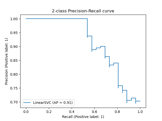
1. sklearn.metrics.precision_recall_curve
- The precision-recall curve shows the tradeoff between precision and recall for different threshold.
1. Binary Classification metrics
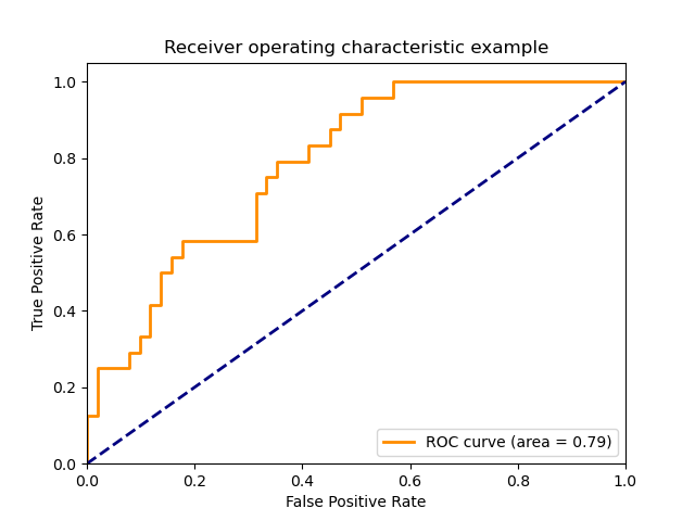
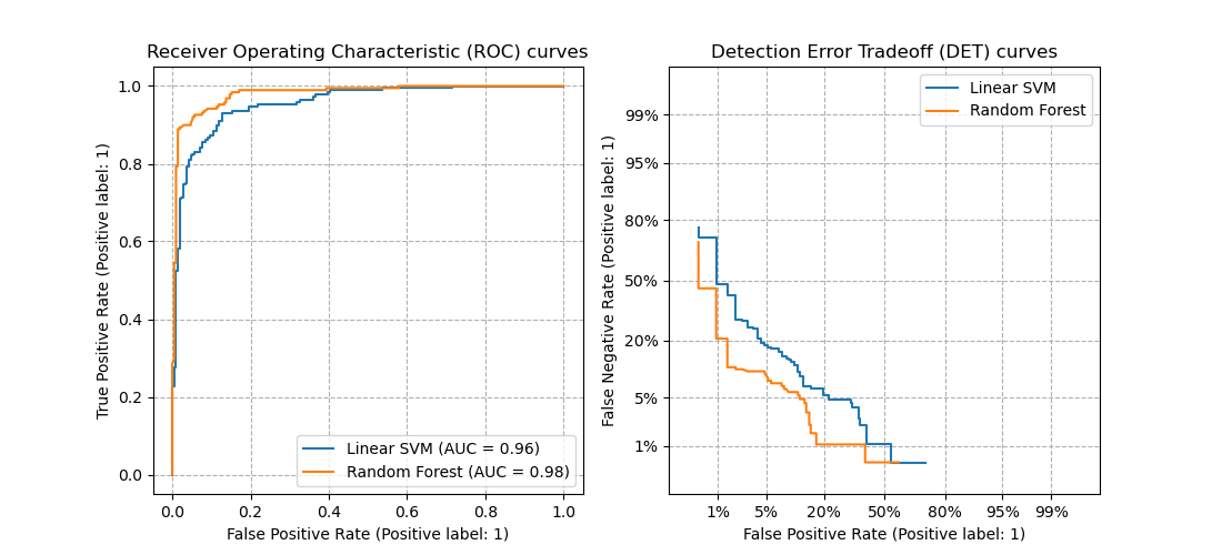
2. sklearn.metrics.roc_curve
- Receiver Operating Characteristic (ROC) curves typically feature true positive rate on the Y axis, and false positive rate on the X axis.
- The top left corner of the plot is the “ideal” point - a false positive rate of zero, and a true positive rate of one.
1. Binary Classification metrics
3. sklearn.metrics.det_curve
- A detection error tradeoff (DET) graph plots false reject rate vs. false accept rate.
- DET curves are a variation of ROC curves where False Negative Rate is plotted on the y-axis instead of True Positive Rate.
1. Binary Classification metrics
- Data is treated as a collection of binary problems, one for each class.
- Binary metric calculations across the set of classes are averaged. Done through the
averageparameter.-
"macro"- calculates the mean of the binary metrics, giving equal weight to each class. -
"weighted"- computes the average of binary metrics in which each class’s score is weighted by its presence in the true data sample. -
"micro"- gives each sample-class pair an equal contribution to the overall metric (except as a result of sample-weight). (preferred in multilabel settings, including multiclass classification where a majority class is to be ignored.) -
"samples"- calculates the metric over the true and predicted classes for each sample in the evaluation data, and returns their (sample_weight-weighted) average. -
"None"will return an array with the score for each class.
-
From binary to multiclass and multilabel
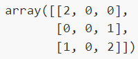
1. sklearn.metrics.confusion_matrix
- This function evaluates classification accuracy by computing the confusion matrix with each row corresponding to the true class.
- By definition, entry \(i,j\) in a confusion matrix is the number of observations actually in group \(i\), but predicted to be in group \(j\).
2. Multiclass Classification metrics
2. sklearn.metrics.balanced_accuracy_score
- Balanced accuracy in binary and multiclass classification problems is defined as the average of recall obtained on each class.
3. sklearn.metrics.cohen_kappa_score
- Cohen’s kappa is a statistic that measures inter-annotator agreement (a score that expresses the level of agreement between two annotators on a classification problem)
4. sklearn.metrics.hinge_loss
- Hinge_loss function computes the average distance between the model and the data using hinge loss, a one-sided metric that considers only prediction errors.
5. sklearn.metrics.matthews_corrcoef
- It is a correlation coefficient value between -1 and +1.
- +1 represents a perfect prediction, 0 an average random prediction and -1 an inverse prediction.
2. Multiclass Classification metrics
6. sklearn.metrics.roc_auc_score
- The toc_auc_score function used in multi-class classification supports two strategies:
- one-vs-one algorithm computes the average of the pairwise ROC AUC scores
- one-vs-rest algorithm computes the average of the ROC AUC scores for each class against all other classes.
7. sklearn.metrics.top_k_accuracy_score
- Computes the number of times where the correct label is among the top k labels predicted (ranked by predicted scores).
2. Multiclass Classification metrics
1. sklearn.metrics.accuracy_score
- In multilabel classification, this function computes subset accuracy: the set of labels predicted for a sample must exactly match the corresponding set of labels in y_true.
2. sklearn.metrics.multilabel_confusion_matrix
- Calculates class-wise or sample-wise multilabel confusion matrices.
- When calculating class-wise multilabel confusion matrix \(C\), the count of true negatives for class \(i\) is \(C_{i,0,0}\), false negatives is \(C_{i,1,0}\), true positives is \(C_{i,1,1}\) and false positives is \(C_{i,0,1}\).
- Example:
3. Multilabel Classification metrics
from sklearn.metrics import multilabel_confusion_matrix
y_true = ["cat", "ant", "cat", "cat", "ant", "bird"]
y_pred = ["ant", "ant", "cat", "cat", "ant", "cat"]
multilabel_confusion_matrix(y_true, y_pred,labels=["ant", "bird", "cat"])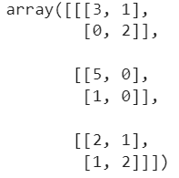
3. sklearn.metrics.classification_report
- This function builds a text report showing the main classification metrics.
- Example:
4. sklearn.metrics.zero_one_loss
-
If
normalizeparameter is True, this function returns the fraction of misclassifications (float), else it returns the number of misclassifications (int).
3. Multilabel Classification metrics
from sklearn.metrics import classification_report
y_true = [0, 1, 2, 2, 0]
y_pred = [0, 0, 2, 1, 0]
target_names = ['class 0', 'class 1', 'class 2']
print(classification_report(y_true, y_pred, target_names=target_names))
4. sklearn.metrics.hamming_loss
- Hamming loss is the fraction of labels that are incorrectly predicted.
- This function computes the average Hamming loss or Hamming distance between two sets of samples.
5. sklearn.metrics.log_loss
- Log loss, also called logistic regression loss or cross-entropy loss, is defined on probability estimates.
- This function computes log loss given a list of ground-truth labels and a probability matrix, as returned by an estimator’s
predict_probamethod.
6. sklearn.metrics.jaccard_score
- The Jaccard index or Jaccard similarity coefficient, defined as the size of the intersection divided by the size of the union of two label sets, is used to compare set of predicted labels for a sample to the corresponding set of labels in
y_true.
3. Multilabel Classification metrics
7. Precision, recall and F-measures
Note: Best value is 1 and the worst value is 0 for these scores.
3. Multilabel Classification metrics
sklearn.metrics.precision_score |
computes precision which is intuitively the ability of the classifier not to label as positive a sample that is negative. |
sklearn.metrics.recall_score |
computes recall which is intuitively the ability of the classifier to find all the positive samples. |
sklearn.metrics.f1_score |
computes harmonic mean of precision and recall |
sklearn.metrics.fbeta_score |
computes weighted harmonic mean of precision and recall |
sklearn.metrics.average_precision_score |
computes the average precision from prediction scores (this score does not supports multiclass) |
8. sklearn.metrics.precision_recall_fscore_support
- Compute precision, recall, F-measure and support for each class.