Linear Regression
Dr. Ashish Tendulkar
Machine Learning Practice
IIT Madras
How to build baseline regression model?
helps in creating a baseline for regression.
DummyRegressor
from sklearn.dummy import DummyRegressor

dummy_regr = DummyRegressor(strategy="mean")
dummy_regr.fit(X_train, y_train)
dummy_regr.predict(X_test)
dummy_regr.score(X_test, y_test)- It makes a prediction as specified by the strategy.
- Strategy is based on some statistical property of the training set or user specified value.
mean
median
quantile
constant
Strategy
quantile
constant
How is Linear Regression model trained?
Normal equation
Iterative optimization
from sklearn.linear_model import LinearRegression
linear_regressor = LinearRegression()
from sklearn.linear_model import SGDRegressor
linear_regressor = SGDRegressor()Step 1: Instantiate object of a suitable linear regression estimator from one of the following two options
Step 2: Call fit method on linear regression object with training feature matrix and label vector as arguments.
# Model training with feature matrix X_train and
# label vector or matrix y_train
linear_regressor.fit(X_train, y_train)
Works for both single and multi-output regression.
SGDRegressor Estimator
SGDRegressor Estimator
- Implements stochastic gradient descent
- Provides greater control on optimization process through provision for hyperparameter settings.
SGDRegressor
-
loss= 'squared error' -
loss = 'huber'
-
penalty = 'l1'
-
penalty = 'l2'
-
penalty = 'elasticnet'
-
learning_rate = 'constant'
-
learning_rate = 'optimal'
-
learning_rate = 'invscaling'
-
learning_rate = 'adaptive'
-
early_stopping = 'True' -
early_stopping = 'False'
- Use for large training set up (> 10k samples)
It's a good idea to use a random seed of your choice while instantiating SGDRegressor object. It helps us get reproducible results.
Set
from sklearn.linear_model import SGDRegressor
linear_regressor = SGDRegressor(random_state=42)
random_state
to seed of your choice.
Note: In the rest of the presentation, we won't set the random seed for sake of brevity. However while coding, always set the random seed in the constructor.
How to perform feature scaling for SGDRegressor?
SGD is sensitive to feature scaling, so it is highly recommended to scale input feature matrix.
from sklearn.linear_model import SGDRegressor
from sklearn.pipeline import Pipeline
from sklearn.preprocessing import StandardScaler

sgd = Pipeline([
		('feature_scaling', StandardScaler())),
        	('sgd_regressor', SGDRegressor())])

sgd.fit(X_train, y_train)- Feature scaling is not needed for word frequencies and indicator features as they have intrinsic scale.
-
Features extracted using PCA should be scaled by some constant \(c\) such that the average L2 norm of the training data equals one.
Note
How to shuffle training data after each epoch in SGDRegressor?
from sklearn.linear_model import SGDRegressor
linear_regressor = SGDRegressor(shuffle=True)
How to use set learning rate in SGDRegreesor?
-
learning_rate = 'constant'
-
learning_rate = 'invscaling'
-
learning_rate = 'adaptive'
What is the default setting?
from sklearn.linear_model import SGDRegressor
linear_regressor = SGDRegressor(random_state=42)-
learning_rate = 'invscaling'
-
eta0 = 1e-2
Learning rate reduces after every iteration: eta = eta0 / pow(t, power_t)
-
power_t = 0.25
Note: You can make changes to these parameters to speed up or slow down the training process.
How to use set constant learning rate ?
-
learning_rate = 'constant'
from sklearn.linear_model import SGDRegressor
linear_regressor = SGDRegressor(learning_rate='constant',
                                eta0=1e-2)
Constant learning rate is used throughout the training.
eta0 = 1e-2
from sklearn.linear_model import SGDRegressor
linear_regressor = SGDRegressor(learning_rate='adaptive',
                                eta0=1e-2)
How to set adaptive learning rate?
-
When the stopping criterion is reached, the learning rate is divided by 5, and the training loop continues.
-
The algorithm stops when the learning rate goes below \(10^{-6}\).
-
The learning rate is kept to initial value as long as the training loss decreases.
How to set #epochs in SGDRegreesor?
from sklearn.linear_model import SGDRegressor
linear_regressor = SGDRegressor(max_iter=100)
Set max_iter to desired #epochs. The default value is 1000.
Remember one epoch is one full pass over the training data.
SGD converges after observing approximately \(10^6\) training samples. Thus, a reasonable first guess for the number of iterations for \(n\) sampled training set is
\text{max\_iter} = \text{np.ceil}(10^6/n)
Practical tip
How to set stopping criteria in SGDRegreesor?
from sklearn.linear_model import SGDRegressor
linear_regressor = SGDRegressor(loss='squared_error',
                                max_iter=500,
                                tol=1e-3,
                                n_iter_no_change=5)
The SGDRegreesor stops
-
when the training loss does not improve (loss > best_loss -
tol)forn_iter_no_changeconsecutive epochs - else after a maximum number of iteration
max_iter.
Option #1
tol, n_iter_no_change, max_iter.
How to set stopping criteria in SGDRegreesor?
The SGDRegreesor stops when
-
validation score does not improve by at least
tolforn_iter_no_changeconsecutive epochs. - else after a maximum number of iteration
max_iter.
Option #2
early_stopping, validation_fraction
from sklearn.linear_model import SGDRegressor
linear_regressor = SGDRegressor(loss='squared_error',
                                early_stopping=True
                                max_iter=500,
                                tol=1e-3,
                                validation_fraction=0.2,
                                n_iter_no_change=5)
Set aside validation_fraction percentage records from training set as validation set. Use score method to obtain validation score.
How to use different loss functions in SGDRegreesor?
from sklearn.linear_model import SGDRegressor
linear_regressor = SGDRegressor(loss='squared_error')
'squared_error'
Set loss parameter to one of the supported values
It also supports other losses as documented in sklearn API
{studied in this course}
How to use averaged SGD?
Averaged SGD updates the weight vector to average of weights from previous updates.
Option #1: Averaging across all updates
average=True
from sklearn.linear_model import SGDRegressor
linear_regressor = SGDRegressor(average=True)
Option #2: Set
from sklearn.linear_model import SGDRegressor
linear_regressor = SGDRegressor(average=10)
average
average=10
to int value.
Averaging begins once the total number of samples seen reaches
average
Setting
starts averaging after seeing 10 samples
Averaged SGD works best with a larger number of features and a higher eta0
How do we initialize SGD with weight vector of the previous run?
Set
warm_start = TRUE
while instantiating object of SGDRegressor
from sklearn.linear_model import SGDRegressor
linear_regressor = SGDRegressor(warm_start=True)
warm_start = False
By default
How to monitor SGD loss iteration after iteration?
sgd_reg = SGDRegressor(max_iter=1, tol=-np.infty, warm_start=True,
                       penalty=None, learning_rate="constant", eta0=0.0005)

for epoch in range(1000):
    sgd_reg.fit(X_train, y_train)  # continues where it left off
    y_val_predict = sgd_reg.predict(X_val)
    val_error = mean_squared_error(y_val, y_val_predict)
Make use of
warm_start = TRUE
Model inspection
How to access the weights of trained Linear Regression model?
linear_regressor.intercept_\(\hat{y} = \color{red}{w_0} \color{black}+ \color{red}{w_1} \color{black}{x_1} + \color{red}{w_2} \color{black}{x_2} + \ldots + \color{red}{w_m} \color{black}{x_m}\) = \( \color{red}{\mathbf{w}^T}\color{black} \mathbf{x}\)
linear_regressor.coef_Note: These code snippets works for both LinearRegression and SGDRegressor, and for that matter to all regression estimators that we will study in this module. Why?
All of them are estimators.
The weights \(\color{red}{w_1, w_2, \ldots, w_m}\) are stored in coef_ class variable.
The intercept \(\color{red}{w_0}\) is stored in intercept_ class variable.
Model inference
How to make predictions on new data in Linear Regression model?
Step 2: Call predict method on linear regression object with feature matrix as an argument.
# Predict labels for feature matrix X_test
linear_regressor.predict(X_test)
Step 1: Arrange data for prediction in a feature matrix of shape (#samples, #features) or in sparse matrix format.
Same code works for all regression estimators.
Model evaluation
STEP 1: Split data into train and test
from sklearn.model_selection import train_test_split
X_train, X_test, y_train, y_test = train_test_split(X, y, random_state=42)
STEP 4: Calculate test error (a.k.a. generalization error)
General steps in model evaluation
STEP 3: Calculate training error (a.k.a. empirical error)
Compare training and test errors
STEP 2: Fit linear regression estimator on training set.
How to evaluate trained Linear Regression model?
Using score method on linear regression object:
# Evaluation on the eval set with
# 1. feature matrix
# 2. label vector or matrix (single/multi-output)
linear_regressor.score(X_test, y_test)
R^2 = \left( 1 - \frac{u}{v}\right)
residual sum of squares:
\(u=(\mathbf{Xw}-\mathbf{y})^T\)\((\mathbf{Xw}-\mathbf{y} )\)
total sum of square
The score returns \(R^2\) or coefficient of determination
\(v =(\mathbf{y}-\mathbf{\hat{y}_{mean}})^T (\mathbf{y}-\mathbf{\hat{y}_{mean}})\)
Sum of squared error (actual and mean predicted label)
Sum of squared error (actual and predicted label)
R^2 = \left( 1 - \frac{u}{v}\right)
The score returns \(R^2\) or coefficient of determination
-
The best possible score is 1.0.
-
The score can be negative (because the model can be arbitrarily worse).
-
A constant model that always predicts the expected value of \(y\), would get a score of 0.0.
\(u\), sum of squared error = 0
When?
\(u = v \)
sklearn provides a bunch of regression metrics to evaluate performance of the trained estimator on the evaluation set.
mean_absolute_error
mean_squarred_error
These metrics can also be used in multi-output regression setup.
r2_score
Same as output of
score
from sklearn.metrics import mean_absolute_error
eval_score = mean_absolute_error(y_test, y_predicted)
from sklearn.metrics import mean_squarred_error
eval_score = mean_squarred_error(y_test, y_predicted)from sklearn.metrics import r2_score
eval_score = r2_score(y_test, y_predicted)Evaluation metrics
mean_squared_log_error
mean_absolute_percentage_error
median_absolute_error
from sklearn.metrics import mean_squared_log_error
eval_score = mean_squared_log_error(y_test, y_predicted)
from sklearn.metrics import mean_absolute_percentage_error
eval_score = mean_absolute_percentage_error(y_test, y_predicted)from sklearn.metrics import median_absolute_error
eval_score = median_absolute_error(y_test, y_predicted)- Useful for targets with exponential growths like population, sales growth etc,
- Penalizes under-estimation heavier than the over-estimation.
- Sensitive to relative error.
- Robust to outliers
How to evaluate regression model on worst case error?
Use metrics
max_error
from sklearn.metrics import max_error
test_error = max_error(y_test, y_predicted)
This metrics can, however, be used only for single output regression. It does not support multi-output regression.
Worst case error on test set can be calculated as follows:
from sklearn.metrics import max_error
train_error = max_error(y_train, y_predicted)
Worst case error on train set can be calculated as follows:
- Score is a metric for which higher value is better.
- Error is a metric for which lower value is better.
Convert error metric to score metric by adding neg_ suffix.
| Function | Scoring |
|---|---|
| metrics.mean_absolute_error | neg_mean_absolute_error |
| metrics.mean_squared_error | neg_mean_squared_error |
| metrics.mean_squared_error | neg_root_mean_squared_error |
| metrics.mean_squared_log_error | neg_mean_squared_log_error |
| metrics.median_absolute_error | neg_median_absolute_error |
Scores and Errors
In case, we get comparable performance on train and test with this split, is this performance guaranteed on other splits too?
-
Is test set sufficiently large?
- In case it is small, the test error obtained may be unstable and would not reflect the true test error on large test set.
-
What is the chance that the easiest examples were kept aside as test by chance?
- This if happens would lead to optimistic estimation of the true test error.
We use cross validation for robust performance evaluation.
Cross-validation performs robust evaluation of model performance
- by repeated splitting and
- providing many training and test errors
This enables us to estimate variability in generalization performance of the model.
ShuffleSplit
KFold
RepeatedKfold
LeaveOneOut
sklearn implements the following cross validation iterators
How to obtain cross validated performance measure using KFold?
from sklearn.model_selection import cross_val_score
from sklearn.linear_model import linear_regression

lin_reg = linear_regression()
score = cross_val_score(lin_reg, X, y, cv=5)- Uses KFold cross validation iterator, that divides training data into 5 folds.
- In each run, it uses 4 folds for training and 1 for evaluation.
from sklearn.model_selection import cross_val_score
from sklearn.model_selection import KFold
from sklearn.linear_model import linear_regression

lin_reg = linear_regression()
kfold_cv = KFold(n_splits=5, random_state=42)
score = cross_val_score(lin_reg, X, y, cv=kfold_cv)
Alternate way of writing the same thing
How to obtain cross validated performance measure using LeaveOneOut?
which is same as
from sklearn.model_selection import cross_val_score
from sklearn.model_selection import LeaveOneOut
from sklearn.linear_model import linear_regression

lin_reg = linear_regression()
loocv = LeaveOneOut()
score = cross_val_score(lin_reg, X, y, cv=loocv)
from sklearn.model_selection import cross_val_score
from sklearn.model_selection import KFold
from sklearn.linear_model import linear_regression
lin_reg = linear_regression()
n = X.shape[0]
kfold_cv = KFold(n_splits=n)
score = cross_val_score(lin_reg, X, y, cv=kfold_cv)How to obtain cross validated performance measure using ShuffleSplit?
from sklearn.linear_model import linear_regression
from sklearn.model_selection import cross_val_score
from sklearn.model_selection import ShuffleSplit

lin_reg = linear_regression()
shuffle_split = ShuffleSplit(n_splits=5, test_size=0.2, random_state=42)
score = cross_val_score(lin_reg, X, y, cv=shuffle_split)
It is also called random permutation based cross validation strategy.
- Generates user defined number of train/test splits.
- It is robust to class distribution.
In each iteration, it shuffles order of data samples and then splits it into train and test.
How to specify a performance measure in
from sklearn.linear_model import linear_regression
from sklearn.model_selection import cross_val_score
from sklearn.model_selection import ShuffleSplit

lin_reg = linear_regression()
shuffle_split = ShuffleSplit(n_splits=5, test_size=0.2, random_state=42)
score = cross_val_score(lin_reg, X, y, cv=shuffle_split,
                        scoring='neg_mean_absolute_error')
parameter can be set to one of the scoring schemes implemented in sklearn as follows
scoring
neg_mean_absolute_error
neg_mean_squared_error
neg_root_mean_squared_error
neg_mean_squared_log_error
neg_median_absolute_error
r2
max_error
cross_val_score
How to obtain test scores from different folds?
from sklearn.model_selection import cross_validate
from sklearn.model_selection import ShuffleSplit

cv = ShuffleSplit(n_splits=40, test_size=0.3, random_state=0)
cv_results = cross_validate(
    regressor, data, target, cv=cv, scoring="neg_mean_absolute_error")
The results are stored in python dictionary with the following keys:
fit_time
score_time
test_score
estimator
train_score
(optional)
(optional)
How to obtain trained estimators and scores on training data during cross validation?
from sklearn.model_selection import cross_validate
from sklearn.model_selection import ShuffleSplit

cv = ShuffleSplit(n_splits=40, test_size=0.3,
                  random_state=0)
cv_results = cross_validate(
    regressor, data, target,
    cv=cv, scoring="neg_mean_absolute_error",
    return_train_score=True,
return_estimator=True)- For trained estimator, set
- For scores on training set, set
return_estimator = True
return_train_score = True
The estimators can be accessed through
estimator
key of the dictionary returned by
cross_validate
How to evaluate multiple metrics of regression in cross validation set up?
from sklearn.model_selection import cross_validate
from sklearn.model_selection import ShuffleSplit

cv = ShuffleSplit(n_splits=40, test_size=0.3,
                  random_state=0)
cv_results = cross_validate(
    regressor, data, target,
    cv=cv,
    scoring=["neg_mean_absolute_error", "neg_mean_squared_error"]
    return_train_score=True,
    return_estimator=True)
allows us to specify multiple scoring metrics
cross_validate
cross_val_score
unlike
How to study effect of #samples on training and test errors?
from sklearn.model_selection import learning_curve

results = learning_curve(
    lin_reg, X_train, y_train, train_sizes=train_sizes, cv=cv,
    scoring="neg_mean_absolute_error")
train_size, train_scores, test_scores = results[:3]
# Convert the scores into errors
train_errors, test_errors = -train_scores, -test_scores
STEP 1: Instantiate an object of learning_curve class with estimator, training data, size, cross validation strategy and scoring scheme as arguments.
STEP 2: Plot training and test scores as function of the size of training sets. And make assessment about model fitment: under/overfitting or right fit.
Underfitting/Overfitting diagnosis
STEP 1: Fit linear models with different number of features.
STEP 2: For each model, obtain training and test errors.
STEP 3: Plot #features vs error graph - one each for training and test errors.
STEP 4: Examine the graphs to detect under/overfitting.
We can replace #features with any other tunable hyperparameter to do this diagnosis for setting that hyperparameter to the appropriate value.
Polynomial regression
How is polynomial regression model trained?
Step 1: Apply polynomial transformation on the feature matrix.
Step 2: Learn linear regression model (via normal equation or SGD) on the transformed feature matrix.
Implementation tips: Make use of pipeline construct for polynomial transformation followed by linear regression estimator.
Step 2: Learn linear regression model (via normal equation or SGD) on the transformed feature matrix.
Set up polynomial regression model with normal equation
from sklearn.linear_model import LinearRegression
from sklearn.pipeline import Pipeline
from sklearn.preprocessing import PolynomialFeatures

# Two steps:
# 1. Polynomial features of desired degree (here degree=2)
# 2. Linear regression
poly_model = Pipeline([
		('polynomial_transform', PolynomialFeatures(degree=2))),
        	('linear_regression', LinearRegression())])

# Train with feature matrix X_train and label vector y_train
poly_model.fit(X_train, y_train)
Set up polynomial regression model with SGD
from sklearn.linear_model import SGDRegressor
from sklearn.pipeline import Pipeline
from sklearn.preprocessing import PolynomialFeatures

poly_model = Pipeline([
		('polynomial_transform', PolynomialFeatures(degree=2))),
        	('sgd_regression', SGDRegressor())])
poly_model.fit(X_train, y_train)
Notice that there is a single line code change in two code snippets.
How to use only interaction features for polynomial regression?
from sklearn.preprocessing import PolynomialFeatures
poly_transform = PolynomialFeatures(degree=2, interaction_only=True)
\([x_1, x_2]\) is transformed to \([1, x_1, x_2, x_1x_2]\).
Note that \([x_1^2, x_2^2]\) are excluded.
Hyperparameter tuning (HPT)
- Hyper-parameters are parameters that are not directly learnt within estimators.
- In sklearn, they are passed as arguments to the constructor of the estimator classes.
How to recognize hyperparameters in any sklearn estimator?
For example,
- degree in PolynomialFeatures
- learning rate in SGDRegressor
How to set these hyperparameters?
Select hyperparameters that results in the best cross validation scores.
Hyper parameter search consists of
- an estimator (regressor or classifier);
- a parameter space;
- a method for searching or sampling candidates;
- a cross-validation scheme; and
- a score function.
Two generic HPT approaches implemented in sklearn are:
param_grid = [
  {'C': [1, 10, 100, 1000], 'kernel': ['linear']}
]- RandomizedSearchCV samples a given number of candidate values from a parameter space with a specified distribution.
- GridSearchCV exhaustively considers all parameter combinations for specified values.
param_dist = {
    "average": [True, False],
    "l1_ratio": stats.uniform(0, 1),
    "alpha": loguniform(1e-4, 1e0),
}
What are the differences between grid and randomized search?
Grid search
Randomized search
Specifies exact values of parameters in grid
Specifies distributions of parameter values and values are sampled from those distributions.
Computational budget can be chosen independent of number of parameters and their possible values.
The budget is chosen in terms of the number of sampled candidates or the number of training iterations. Specified in n_iter argument
What data split is recommended for HPT?

What are the steps in HPT?
STEP 1: Divide training data into training, validation and test sets.
STEP 2: For each combination of hyper-parameter values learn a model with training set.

This step creates multiple models.
- This step can be be run in parallel by setting n_jobs = -1.
- Some parameter combinations may cause failure in fitting one or more folds of data. This may cause the search to fail. Set error_score = 0 (or np.NaN) to set score for the problematic fold to 0 and complete the search.
Tips
STEP 3: Evaluate performance of each model with validation set and select a model with the best evaluation score.


STEP 4: Retrain model with the best hyper-parameter settings on training and validation set combined.
STEP 5: Evaluate the model performance on the test set.

Note that the test set was not used in hyper-parameter search and model retraining .
What are some of model specific HPT available for regression tasks?
-
Some models can fit data for a range of values of some parameter almost as efficiently as fitting the estimator for a single value of the parameter.
-
This feature can be leveraged to perform more efficient cross-validation used for model selection of this parameter.
- linear_model.LassoCV
- linear_model.RidgeCV
- linear_model.ElasticNetCV
How to determine degree of polynomial regression with grid search?
from sklearn.model_selection import GridSearchCV
from sklearn.pipeline import Pipeline
from sklearn.preprocessing import POlynomialFeatures
from sklearn.linear_model import SGDRegressor

param_grid = [
    {'poly__degree': [2, 3, 4, 5, 6, 7, 8, 9]}
  ]

pipeline = Pipeline(steps=[('poly', PolynomialFeatures()),
                           ('sgd', SGDRegressor())])

grid_search = GridSearchCV(pipeline, param_grid, cv=5,
                           scoring='neg_mean_squared_error',
                           return_train_score=True)

grid_search.fit(x_train.reshape(-1, 1), y_train)
Regularization
How to perform ridge regularization with specific regularization rate?
fit, score, predict work exactly like other linear regression estimators
from sklearn.linear_model import Ridge
ridge = Ridge(alpha=1e-3)
Step 1: Instantiate object of Ridge estimator
Step 2: Set parameter alpha to the required regularization rate.
[Option #1]
[Option #2]
from sklearn.linear_model import SGDRegressor
sgd = SGDRegressor(alpha=1e-3, penalty='l2')
Step 1: Instantiate object of SGDRegressor estimator
Step 2: Set parameter alpha to the required regularization rate and penalty = l2.
How to search the best regularization parameter for ridge?
Search for the best regularization rate with built-in cross validation in RidgeCV estimator.
[Option #1]
Use cross validation with Ridge or SVDRegressor to search for best regularization.
[Option #2]
- Grid search
- Randomized search
from sklearn.linear_model import Ridge
from sklearn.pipeline import Pipeline
from sklearn.preprocessing import PolynomialFeatures

poly_model = Pipeline([
		('polynomial_transform', PolynomialFeatures(degree=2))),
        	('ridge', Ridge(alpha=1e-3))])
poly_model.fit(X_train, y_train)
How to perform ridge regularization in polynomial regression?
Set up a pipeline of polynomial transformation followed by the ridge regressor.
Instead of Ridge, we can use SGDRegressor, as shown on previous slide, to get equivalent formulation.
How to perform lasso regularization with specific regularization rate?
fit, score, predict work exactly like other linear regression estimators
from sklearn.linear_model import Lasso
lasso = Lasso(alpha=1e-3)
Step 1: Instantiate object of Lasso estimator
Step 2: Set parameter alpha to the required regularization rate.
[Option #1]
[Option #2]
from sklearn.linear_model import SGDRegressor
sgd = SGDRegressor(alpha=1e-3, penalty='l1')
Step 1: Instantiate object of SGDRegressor estimator
Step 2: Set parameter alpha to the required regularization rate and penalty = l1.
How to search the best regularization parameter for lasso regularization?
Search for the best regularization rate with built-in cross validation in LassoCV estimator.
[Option #1]
Use cross validation with Lasso or SVDRegressor to search for best regularization.
[Option #2]
- Grid search
- Randomized search
from sklearn.linear_model import Lasso
from sklearn.pipeline import Pipeline
from sklearn.preprocessing import PolynomialFeatures

poly_model = Pipeline([
		('polynomial_transform', PolynomialFeatures(degree=2))),
        	('lasso', Lasso(alpha=1e-3))])
poly_model.fit(X_train, y_train)
How to perform lasso regularization in polynomial regression?
Set up a pipeline of polynomial transformation followed by the lasso regressor.
Instead of Lasso, we can use SGDRegressor to get equivalent formulation.
from sklearn.linear_model import Lasso
from sklearn.pipeline import Pipeline
from sklearn.preprocessing import PolynomialFeatures

poly_model = Pipeline([
		('polynomial_transform', PolynomialFeatures(degree=2))),
        	('elasticnet', SGDRegressor(penalty='elasticnet',
                                        l1_ratio=0.3))])
poly_model.fit(X_train, y_train)
How to perform both lasso and ridge regularization in polynomial regression?
Set up a pipeline of polynomial transformation followed by the SGDRegressor with
Remember elasticnet is a convex combination of L1 (Lasso) and L2 (Ridge) regularization.
- In this example, we have set l1_ratio to 0.3, which means l2_ratio = 1- l1_ratio = 0.7. L2 takes higher weightage in this formulation.
penalty = 'elasticnet'
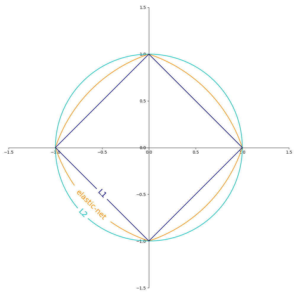
Illustration of L1, L2 and ElasticNet regularizations
Source: sklearn user guide
Summary
How to implement
- Different regression models: standard linear regression and polynomial regression.
- Regularization.
- Model evaluation through different error metrics and scores derived from them.
- Cross validation - different iterators
- Hyperparameter tuning via grid search and randomized search.
Appendix - More Details
Introduction
In this module, we will be covering the implementation aspects of models of linear regression.
First we will learn linear regression models with:
-
Normal equation, which estimates model parameter with a closed-form solution.
-
Iterative optimization approach of gradient descent and its variants namely batch, mini-batch and stochastic gradient descent.
- Since the polynomial regression uses more parameters (due to polynomial representation of the input), it is more prone to overfitting.
- We will study how to detect overfitting with learning curves and use of regularization to mitigate the risk of overfitting.
Further, we will study the implementation of the polynomial regression model, that is capable of modelling non-linear relationships between features and labels.
Recap
Let's recall components of Linear regression
Training Data
(features, label) or \((\color{blue}{X}, \color{red}{y} \color{black}{)} \), where label \(\color{red}{y}\) is a real number.
Model
\(\hat{y} = \color{red}{w_0} \color{black}+ \color{red}{w_1} \color{black}{x_1} + \color{red}{w_2} \color{black}{x_2} + \ldots + \color{red}{w_m} \color{black}{x_m}\) = \( \color{red}{\mathbf{w}^T}\color{black} \mathbf{x}\)
where,
- \(\hat{y}\) is the predicted value.
-
\( \mathbf{X}\) is a feature vector \(\{x_1, x_2, \ldots, x_m\} \) for a given example with \(m \) features in total.
- \( \color{black}{i}\)-th feature: \(x_i \)
- Weight or parameter vector \( \mathbf{\color{red}{w}}\) includes bias term too: \( \{\color{red}{w_0, w_1, w_2, \ldots, w_m}\color{black}\} \)
-
\(\color{red}{w_i}\) is \(i\)-the model parameter associated with \(i\)-the feature.
-
\(h_{\mathbf{\color{red}{w}}}\) is a model with parameter vector \(\mathbf{\color{red}{w}}\).
The label is obtained by a linear combination (or weighted sum) of the input features and a bias (or intercept) term. The model \(h_\mathbf{w}\) is given by
Loss function
J(\mathbf{w})= \dfrac{1}{2} \sum\limits_{i=1}^{n} \left (\hat{y}^{(i)} \color{black} - \color{blue}{y^{(i)}} \color{black}\right )^2\\
\\
J(\mathbf{w})= \dfrac{1}{2} \sum\limits_{i=1}^{n} \left (\color{red}{\mathbf{w}^T \mathbf{x}^{(i)}} \color{black} - \color{blue}{y^{(i)}} \color{black}\right )^2
The model parameters \( \mathbf{\color{red}{w}}\) are learnt such that the square of difference between the actual and the predicted values is minimized.
Optimization
- Normal equation
- Iterative optimization with gradient descent: full batch, mini-batch or stochastic.
Evaluation measure
- Mean squared error
- Root mean squared error
Implementing with sklearn
Normal equation
from sklearn.linear_model import LinearRegressionsklearn provides LinearRegression estimator for weight vector estimation via normal equation
lin_reg = LinearRegression(normalize=True)
lin_reg.fit(X_train, y_train)
It's a good practice to scale or normalize features. We can set normalize flag to True for normalizing the input features.
By default, normalize is False.
As like other estimator object, it implements fit method that takes dataset as an input along with any other hyperparameters and returns estimated weight vector.
It also implements a couple of other methods:
- predict: Predicts label for a new examples based on the learnt model.
- score: Returns \(R^2\) of the linear regression model.
Coefficient of determination \(R^2\)
R^2 = \left( 1 - \frac{u}{v}\right)
where
-
\(u\) is the residual sum of squares and is calculated as
\(u=(\mathbf{Xw}-\mathbf{y})^T\)\((\mathbf{Xw}-\mathbf{y} )\)
-
and \(v\) is the total sum of square. Let, \(\hat{y}_{mean} =\frac{1}{n} \left(\mathbf{Xw}\right) \), then \(v\) is calculated as
\(v =(\mathbf{y}-\mathbf{\hat{y}_{mean}})^T (\mathbf{y}-\mathbf{\hat{y}_{mean}})\)
-
The best possible score is 1.0.
-
The score can be negative (because the model can be arbitrarily worse).
-
A constant model that always predicts the expected value of \(y\), disregarding the input features, would get a score of 0.0.
R^2 = \left( 1 - \frac{u}{v}\right)
Since we generated data with the following equation:
\(y = 4 + 3x_1+noise\),
we know actual values of the parameters: \(\color{red}{w_0} \color{black} =4\) and \( \color{red}{w_1} \color{black}= 3\).
We can compare these values with the estimated values. Note that we do not have this luxury in real world problems, since we do not have access to the data generation process and its parameters.
There we rely on the evaluation metrics to assess quality of the model.
Model inspection
The learnt weights can be obtained by accessing the following class variables of LinearRegression estimator:
-
The intercept weight \(\color{red}{w_0}\) can be obtained via
intercept_class variable.
-
The weights can be obtained via
coef_class variable.
lin_reg.intercept_, lin_reg.coef_Model inspection
Computational Complexity
-
The normal equation uses the following equation to obtain
\(\mathbf{\color{red}{w}} = \left(\mathbf{X}^T\mathbf{X}\right)^{-1}\mathbf{X}^T\mathbf{y}\)
-
This involves matrix inversion operation of feature matrix \(\mathbf{X}\).
-
The `LinearRegression`estimator uses SVD for this task and has the complexity of \(O(m^2)\) where \(m\) is the number of features.
This implies that if we double the number of features, the training computation grows roughly 4 times.
-
As the number of features grows large, the approach of normal equation slows down significantly.
-
These approaches are linear w.r.t. the number of training examples as long as the training set fits in the memory.
-
The inference process is linear w.r.t. both the number of examples and number of features.
Weight vector estimation via SGD
-
SGD is a simple yet very efficient approach of learning weight vectors in linear regression problems especially in large scale problem settings.
-
SGD offers provisions for tuning the optimization process. However as a downside of this, we need to set a few hyperparameters.
-
SGD is sensitive to feature scaling.
In sklearn, an estimator SGDRegressor implements a plain stochastic gradient descent learning routine which supports different loss functions and penalties to fit linear regression models.
-
SGDRegressor is well suited for regression problems with a large number of training samples (> 10,000). For learning problems with small number of training examples, sklearn user guide recommends Ridge or Lasso.
Key functionalities of SGDRegressor
Loss function:
-
Can be set via the loss parameter.
-
SGDRegressor supports the following loss functions.
-
loss= 'squared error': Ordinary least squares, -
loss = 'huber': Huber loss for robust regression
-
Regularization
SGD supports the following penalties:
-
Penalty = 'l2': L2 norm penalty oncoef_. This is default setting.
-
penalty = 'l1': L1 norm penalty oncoef_. This leads to sparse solutions.
-
penalty = 'elasticnet': Convex combination of L2 and L1;
`(1 - l1_ratio) * L2 + l1_ratio * L1
The learning rate \(\eta\) can be either constant or gradually decaying. There are following options for learning rate schedule specification in SGD:
Learning rate
For regression the default learning rate schedule is inverse scaling learning_rate = 'invscaling'. The learning rate in \(t\)-th iteration or time step is calculated as
\(\color{blue}{\eta}^{\color{black}{(t)}} \color{black}= \frac{\eta_0}{t^{power\_t}}\)
where, \(\eta_0\) and power_t are hyperparameters chosen by the user.
1. invscaling
2. Constant
For a constant learning rate use learning_rate = 'constant' and use \(\eta_0\) to specify the learning rate.
3. Adaptive
For an adaptively decreasing learning rate, use learning_rate = 'adaptive' and use \(\eta_0\) to specify the starting learning rate.
-
When the stopping criterion is reached, the learning rate is divided by 5, and the training loop continues.
The algorithm stops when the learning rate goes below \(10^{-6}\).
4. Optimal
Used as a default setting for classification problems. The learning rate \(\eta\) for \(t\)-th iteration is calculated as follows:
\(\eta^{(t)} = \dfrac{1}{\alpha(t_0+t)}\)
Here
-
\(\alpha\) is a regularization rate.
-
\(t\) is the time step (there are a total of
n_samples*n_itertime steps)
-
\(t_0\) is determined based on a heuristic proposed by Léon Bottou such that the expected initial updates are comparable with the expected size of the weights (this assuming that the norm of the training samples is approx. 1).
Stoping creteria
SGDRegressor provides two stopping criteria to stop the algorithm when a given level of convergence is reached:
1. With early_stopping = True
-
The input data is split into a training set and a validation set based on the
validation_fractionparameter.
-
The model is fitted on the training set, and the stopping criterion is based on the prediction score (using the scoring method) computed on the validation set.
2. With early_stopping = False
The model is fitted on the entire input data and
The stopping criterion is based on the objective function computed on the training data.
- In both cases, the criterion is evaluated once by epoch, and the algorithm stops when the criterion does not improve
n_iter_no_change timesin a row.
- The improvement is evaluated with absolute tolerance
tol. - The algorithm stops in any case after a maximum number of iteration
max_iter
SGDRegressor supports averaged SGD (ASGD). Averaging can be enabled by setting average = True
-
ASGD performs the same updates as the regular SGD, and sets
coef_attribute to the average value of the coefficients across all updates.-
SGD sets
coef_attribute to the last value of the coefficients (i.e. the values of the last update)
-
SGD variation: Average SGD
-
The same process is followed for the
intercept_attribute.
When using ASGD the learning rate can be larger and even constant, leading to a speed up in training.
Model inspection
We obtain the weight vector from the trained model as follows:
-
coef_variable stores weights assigned to the features.
-
intercept_, as name suggests, stores the intercept term.
Complexity
The major advantage of SGD is its efficiency, which is basically linear in the number of training examples.
Recent theoretical results, however, show that the runtime to get some desired optimization accuracy does not increase as the training set size increases.
If \(\mathbf{X}\) is a matrix of size \((n, m)\) training has a cost of \(O(knp)\).
-
where \(k\) is the number of iterations (epochs) and \(p\) is the average number of non-zero attributes per sample.
Polynomial regression
Polynomial regression
Polynomial regression = Polynomial transformation + Linear Regression
PolynomialFeatures transformer transforms an input data matrix into a new data matrix of a given degree.
Example:
from sklearn.preprocessing import PolynomialFeatures
import numpy as np
X = np.arange(6).reshape(3, 2)
print ("Data matrix: \n", X)
poly = PolynomialFeatures(degree=2)
print ("\n\nAfter transformation: \n", poly.fit_transform(X))
Data matrix:
[[0 1]
[2 3]
[4 5]]
After transformation:
[[ 1. 0. 1. 0. 0. 1.]
[ 1. 2. 3. 4. 6. 9.]
[ 1. 4. 5. 16. 20. 25.]]Output:
In the above example, the features of \(\mathbf{X}\) have been transformed from \([x_1,x_2]\) to \(\left[ 1, x_1, x_2, x_1^2, x_1x_2, x_2^2 \right]\), and can now be used within any linear model.
In some cases it’s not necessary to include higher powers of any single feature, but only the so-called interaction features that multiply together as most distinct features. These can be gotten from 'PolynomialFeatures' with the setting interaction_only = True.
In this case, the features of \(\mathbf{X}\) would be transformed from \([x_1, x_2]\) to \(\left[ 1, x_1, x_2, x_1x_2 \right]\).
Ridge regression
Ridge regression minimizes \(L_2\) penalized sum of squared error.
Ridge regression
Ridge Loss = Sum of squared error + regularization_rate * penalty
We use 'Ridge' estimator for implementing ridge regression. It takes parameter 'alpha' which is the regularization rate.
-
'RidgeCV' estimator implements ridge regression with cross validation for regularization rate.
RidgeCV parameters:
-
alphasis the list of regularization rates to try.
-
The regularization rate must be positive.
-
Larger values indicate stronger regularization.
2. cv determines the cross-validation splitting strategy.
-
None, to use the efficient Leave-One-Out cross-validation -
integer, to specify the number of folds. -
CV splitterspecifies how to generate cross validation sets. An iterable yielding (train, test) splits as arrays of indices.
In case of a binary or multiclass problems, for 'cv=None' or 'cv=5' (i.e. integer), 'StratifiedKFold' cross validation strategy is used. In other cases, 'KFold' cross validation strategy is used.
Model inspection
'RidgeCV' provides an additional output apart from usual outputs like coef_ and intercept_:
-
alphasprovides the estimated regularization parameter.
Lasso regression
Lasso regression
Lasso uses \(L1\) norm of weight vector as a penalty in linear regression loss function.
'sklearn' provides two implementations for learning weight vector in Lasso.
-
'Lasso' uses coordinated descent algorithm.
-
'LassoLars' uses least angle regression algorithm. It is adaption of forward stepwise feature selection for solving Lasso regression.
Backup MLP 3 & 4 Linear regression
By Swarnim POD


