Data Preprocessing

Machine Learning Practice

Dr. Ashish Tendulkar

IIT Madras

The real world training data is usually not clean and has many issues such as missing values for certain features, features on different scales, non-numeric attributes etc.

Often there is a need to pre-process the data to make it amenable for training the model.

The same pre-processing should be applied to both training and test set.

Sklearn provides pipeline for making it easier to chain multiple transforms together and apply them uniformly across train, eval and test sets.

Sklearn provides a rich set of transformers for this job.

Once you get the training data, the first job is to explore the data and list down preprocessing needed.

Typical problems include

Missing values in features

Numerical features are not on the same scale.

Categorical attributes need to be represented with sensible numerical representation.

Too many features, reduce them.

Extract features from non-numeric data.

Sklearn provides a library of transformers for data preprocessing.

Data cleaning (sklearn.preprocessing) such as standardization, missing value imputation, etc.
Feature extraction (sklearn.feature_extraction)
Feature reduction (sklearn.decomposition.pca)
Feature expansion (sklearn.kernel_approximation)

fit() method learns model parameters from a training set.

Each transformer has the following methods:

transform() method applies the learnt transformation to the new data.

fit_transform() performs function of both fit() and transform() methods and is more convenient and efficient to use.

Transformer methods

Part 1. Feature extraction

FeatureHasher

DictVectorizer

sklearn.feature_extraction has useful APIs to extract features from data:

Let's study these APIs one by one.

DictVectorizer

Converts lists of mappings of feature name and feature value, into a matrix.

\mathbf{X'}_{4 \times 2} = \begin{bmatrix} 4 & 96.0\\ 1 & 73.9\\ 3 & 88.9\\ 2 & 81.6\\ \end{bmatrix}

Original data

Transformed feature matrix \(\mathbf{X'}\)

dv = DictVectorizer(sparse=False)
dv.fit_transform(data)

data =

[{'age': 4, 'height':96.0},

{'age': 1, 'height':73.9},

{'age': 3, 'height':88.9},

{'age': 2, 'height':81.6}]

FeatureHasher

High-speed, low-memory vectorizer that uses feature hashing technique.
Instead of building a hash table of the features, as the vectorizers do, it applies a hash function to the features to determine their column index in sample matrices directly.
This results in increased speed and reduced memory usage, at the expense of inspectability; the hasher does not remember what the input features looked like and has no inverse_transform method.
Output of this transformer is scipy.sparse matrix.

sklearn.feature_extraction.image.* has useful APIs to extract features from image data. Find out more about them in sklearn user guide at the following link: Feature Extraction from Images.

Feature Extraction from images and text

sklearn.feature_extraction.text.* has useful APIs to extract features from text data. Find out more about them in sklearn user guide at the following link: Feature Extraction from Text.

Part 2: Data Cleaning

Handling missing values

Missing values occur due to errors in data capture such as sensor malfunctioning, measurement errors etc.

Discarding records containing missing values would result in loss of valuable training samples.

Many ML algorithms do not work with missing data and need all features to be present.

sklearn.impute API provides functionality to fill missing values in a dataset.

SimpleImputer

KNNImputer

provides indicators for missing values.

MissingIndicator

SimpleImputer

Fills missing values with one of the following strategies: 'mean', 'median', 'most_frequent' and 'constant'.

\mathbf{X}_{4 \times 2} = \begin{bmatrix} 7 & 1\\ \color{red}{nan} & 8\\ 2 & \color{red}{nan}\\ 9 & 6\\ \end{bmatrix}

\mathbf{X'}_{4 \times 2} = \begin{bmatrix} 7 & 1\\ \color{red}6 & 8\\ 2 & \color{red}5\\ 9 & 6\\ \end{bmatrix}

Original feature matrix \(\mathbf{X}\)

Transformed feature matrix \(\mathbf{X'}\)

si = SimpleImputer(strategy='mean')
si.fit_transform(X)

\(\dfrac{7+2+9}{3} = 6\)

\(\dfrac{1+8+6}{3} = 5\)

KNNImputer

Uses k-nearest neighbours approach to fill missing values in a dataset.
- The missing value of an attribute in a specific example is filled with the mean value of the same attribute of n_neighbors closest neighbors.
The nearest neighbours are decided based on Euclidean distance.

Example: KNNImputer

Consider following feature matrix.

\mathbf{X}_{4 \times 3} = \begin{bmatrix} 1. & 2. & nan \\ 3. & 4. & 3. \\ nan & 6. & 5. \\ 8. & 8. & 7. \\ \end{bmatrix}

It has 4 samples and 2 missing values.

Let's fill in missing values with KNNImputer.

\(\text{dist}(x,y) = \sqrt{\text{weight }\times \text{distance from present coordinates}^2}\)

Computing Euclidean distance in presence of missing values

\(\text{weight} = \dfrac{\text{total number of coordinates}}{\text{number of present coordinates}}\)

For example, the distance between \(x= [3, nan, nan, 6]\) and \(y = [1, nan, 4, 5]\) is:

\text{dist}(x,y) = \sqrt{ 2 \times 5} \approx 3.3

\(\text{weight} = \dfrac{\text{total number of coordinates}}{\text{number of present coordinates}} = \dfrac{\text{4}}{\text{2}} = 2\)

\(\text{distance from present coordinates}^2 = (3-1)^2+ (6-5)^2 = 5\)

Let's fill the missing value in first sample/row.

\begin{bmatrix} 3. & 4. & 3. \\ \end{bmatrix}

\begin{bmatrix} nan & 6. & 5. \\ \end{bmatrix}

\begin{bmatrix} 8. & 8. & 7. \\ \end{bmatrix}

Distance with \([1. \quad 2. \quad nan.]\)

\sqrt{ \frac{3}{2}((1-3)^2+ (2-4)^2)} \approx 3.46

\sqrt{\frac{3}{2}((1-8)^2+ (2-8)^2)} \approx 11.29

\(2\) nearest neighbours

\([1. \quad 2. \quad \color{red}{4.} \color{black}]\)

\(\dfrac{3+5}{2}=4\)

# of neighbours

Values of the feature from \(2\) nearest neighbours

\mathbf{X}_{4 \times 3} = \begin{bmatrix} 1. & 2. & nan \\ 3. & 4. & 3. \\ nan & 6. & 5. \\ 8. & 8. & 7. \\ \end{bmatrix}

% \sqrt{\frac{3}{2}((1-8)^2+ (2-8)^2)} \approx 9.21 % \sqrt{ \frac{3}{1}(2-6)^2} \; \;\;\;\;\qquad \qquad \approx 6.92

\mathbf{X'}_{4 \times 4} = \begin{bmatrix} 1. & 2. & \color{red}4. \\ 3. & 4. & 3. \\ \color{red}5.5 & 6. & 5. \\ 8. & 8. & 7. \\ \end{bmatrix}

\mathbf{X}_{4 \times 4} = \begin{bmatrix} 1. & 2. & nan. \\ 3. & 4. & 3. \\ nan & 6. & 5. \\ 8. & 8. & 7. \\ \end{bmatrix}

knni = KNNImputer(n_neighbors=2, weights="uniform")
knni.fit_transform(X)

Original feature matrix \(\mathbf{X}\)

Transformed feature matrix \(\mathbf{X'}\)

In this way, we can fill up the missing values with KNNImputer.

Marking imputed values

It is useful to indicate the presence of missing values in the dataset.
MissingIndicator helps us get those indications.
- It returns a binary matrix,
  - True values correspond to missing entries in original dataset.

1.2 Numeric transformers

Feature scaling
Polynomial transformation
Discretization

Let's learn how to scale numerical features with sklearn API.

Feature scaling

Numerical features with different scales leads to slower convergence of iterative optimization procedures.

It is a good practice to scale numerical features so that all of them are on the same scale.

MaxAbsScaler

MinMaxScaler

StandardScaler

Three feature scaling APIs are available in sklearn

StandardScaler

\(\mathbf{x'} = \dfrac{\mathbf{x}-\mu}{\sigma}\)

Transforms the original features vector \(\mathbf{x}\) into new feature vector \(\mathbf{x'}\) using following formula

\mathbf{x}_{5 \times 1} = \begin{bmatrix} 4 \\ 3 \\ 2 \\ 5 \\ 6 \\ \end{bmatrix}

\(\mu = 4, \sigma = \sqrt 2\)

\mathbf{x'}_{5 \times 1} = \begin{bmatrix} 0 \\ -1/\sqrt 2 \\ -2/\sqrt 2 \\ 1/\sqrt 2 \\ 2/\sqrt 2 \\ \end{bmatrix}

\(\mu' = 0, \sigma '= 1\)

ss = StandardScalar()
ss.fit_transform(x)

Note that the transformed feature vector \(\mathbf{x'}\) has mean (\(\mu\)) = 0 and standard deviation (\(\sigma\)) = 1.

Learns parameters \(\mu\) and \(\sigma\).

\(\mathbf{x'} = \dfrac{\mathbf{x}-\mathbf{x}.min}{\mathbf{x}.max - \mathbf{x}.min}\)

It transforms the original feature vector \(\mathbf{x}\) into new feature vector \(\mathbf{x'}\) so that all values fall within range \([0,\ 1]\)

where \(\mathbf{x}.max\) and \(\mathbf{x}.min\) are largest and smallest values of that feature respectively, of the original feature vector \(\mathbf{x}\).

MinMaxScaler

\mathbf{x'}_{5 \times 1} = \begin{bmatrix} 1 \\ 0.35 \\ 0.5 \\ 0.6 \\ 0 \\ \end{bmatrix}

\mathbf{x}_{5 \times 1} = \begin{bmatrix} 15 \\ 2 \\ 5 \\ -2 \\ -5\\ \end{bmatrix}

mms = MinMaxScalar()
mms.fit_transform(x)

\(\mathbf{x}.max\) = 15, \(\mathbf{x}.min\) = -5

The largest number is transformed to 1 and the smallest number is transformed to 0.

\(\mathbf{x'} = \dfrac{\mathbf{x}}{\text{MaxAbsoluteValue}}\)

It transforms the original features vector \(\mathbf{x}\) into new feature vector \(\mathbf{x'}\) so that all values fall within range \([-1,\ 1]\)

where \(\text{MaxAbsoluteValue} = \text{max}(\mathbf{x}.max, |\mathbf{x}.min|)\)

MaxAbsScaler

\mathbf{x'}_{5 \times 1} = \begin{bmatrix} 0.04 \\ 0.02 \\ 0.05 \\ -0.02 \\ -1 \\ \end{bmatrix}

\mathbf{x}_{5 \times 1} = \begin{bmatrix} 4 \\ 2 \\ 5 \\ -2 \\ -100\\ \end{bmatrix}

mas = MaxAbsScalar()
mas.fit_transform(x)

\(\text{MaxAbsoluteValue}\) = \(\text{max}(5, |-100|) = 100\)

Constructs transformed features by applying a user defined function.

FunctionTransformer

\mathbf{X'}_{4 \times 2} = \begin{bmatrix} 7 & 1\\ 1 & 8\\ 2 & 0\\ 9 & 6\\ \end{bmatrix}

\mathbf{X}_{4 \times 2} = \begin{bmatrix} 128 & 2\\ 2 & 256\\ 4 & 1\\ 512 & 64\\ \end{bmatrix}

ft = FunctionTransformer(numpy.log2)
ft.fit_transform(X)

Applies \(\text{log}_2\) function to the features.

Polynomial transformation

Generates a new feature matrix consisting of all polynomial combinations of the features with degree less than or equal to the specified degree.

\(\mathbf{X'} = [\mathbf{x}_1, \mathbf{x}_2, \mathbf{x}_1 \mathbf{x}_2, \mathbf{x}^2_1, \mathbf{x}^2_2] \)

\(\mathbf{X'} = [\mathbf{x}_1, \mathbf{x}_2, \mathbf{x}_1\mathbf{x}_2, \mathbf{x}^2_1, \mathbf{x}^2_2, \mathbf{x}^2_1\mathbf{x}_2, \mathbf{x}_1\mathbf{x}^2_2, \mathbf{x}^3_1, \mathbf{x}^3_2] \)

\(\mathbf{X}=[\mathbf{x}_1, \mathbf{x}_2] \)

degree =\(2\)

pf=PolynomialFeatures(degree=2)
pf.fit_transform(X)

pf=PolynomialFeatures(degree = 3)
pf.fit_transform(X)

degree =\(3\)

Divides a continuous variable into bins.
One hot encoding or ordinal encoding is further applied to the bin labels.

\mathbf{x}_{9 \times 1} = \begin{bmatrix} 0\\ 0.125\\ 0.25\\ 0.375\\ 0.5\\ 0.675\\ 0.75\\ 0.875\\ 1.0\\ \end{bmatrix}

KBinsDiscretizer

\mathbf{x'}_{9 \times 1} = \begin{bmatrix} 0. \\ 0. \\ 1. \\ 1. \\ 2. \\ 3. \\ 3. \\ 4. \\ 4. \\ \end{bmatrix}

KBinsDiscretizer(
  n_bins=5, 
  strategy='uniform', 
  encode = 'ordinal')

1.2 Categorical transformers

Feature encoding
Label encoding

OneHotEncoder

Encodes categorical feature or label as a one-hot numeric array.
Creates one binary column for each of \(K\) unique values.
Exactly one column has 1 in it and rest have 0.

\mathbf{x}_{4 \times 1} = \begin{bmatrix} 1 \\ 2 \\ 3 \\ 1 \\ \end{bmatrix}

\mathbf{X'}_{4 \times 3} = \begin{bmatrix} 1 & 0 & 0 \\ 0 & 1 & 0 \\ 0 & 0 & 1 \\ 1 & 0 & 0 \\ \end{bmatrix}

# unique values: \(K=3\)

ohe=OneHotEncoder()
ohe.fit_transform(x)

# columns in transformed matrix = 3

LabelEncoder

Encodes target labels with value between 0 and \(K -1\), where \(K\) is number of distinct values.

Here \(K=4\): \(\{1, 2, 6, 8\}\)

\mathbf{y}_{6 \times 1} = \begin{bmatrix} 1 \\ 2 \\ 6 \\ 1 \\ 8 \\ 6\\ \end{bmatrix}

\mathbf{y'}_{6 \times 1} = \begin{bmatrix} 0 \\ 1 \\ 2 \\ 0 \\ 3 \\ 2 \\ \end{bmatrix}

le = LabelEncoder()
le.fit_transform(y)

1 is encoded as 0, 2 as 1, 6 as 2, and 8 as 3.

OrdinalEncoder

Encodes categorical features with value between 0 and \(K -1\), where \(K\) is number of distinct values.

OrdinalEncoder can operate multi dimensional data, while LabelEncoder can transform only 1D data.

\mathbf{X}_{6 \times 2} = \begin{bmatrix} 1 & \lq{male}\rq\\ 2 & \lq{female}\rq\\ 6 & \lq{female}\rq\\ 1 & \lq{male}\rq\\ 8 & \lq{male}\rq\\ 6 & \lq{female}\rq\\ \end{bmatrix}

\mathbf{X'}_{6 \times 2} = \begin{bmatrix} 0 & 1\\ 1 & 0\\ 2 & 0\\ 0 & 1\\ 3 & 1\\ 2 & 0\\ \end{bmatrix}

oe = OrdinalEncoder()
oe.fit_transform(X)

LabelBinarizer

\mathbf{y}_{6 \times 1} = \begin{bmatrix} 1 \\ 2 \\ 6 \\ 1 \\ 8 \\ 6\\ \end{bmatrix}

\mathbf{Y'}_{6 \times 4} = \begin{bmatrix} 1 & 0 & 0 & 0 \\ 0 & 1 & 0 & 0 \\ 0 & 0 & 1 & 0 \\ 1 & 0 & 0 & 0 \\ 0 & 0 & 0 & 1 \\ 0 & 0 & 1 & 0 \\ \end{bmatrix}

lb=LabelBinarizer()
lb.fit_transform(y)

Several regression and binary classification can be extended to multi-class setup in one-vs-all fashion.

This involves training a single regressor or classifier per class.

For this, we need to convert multi-class labels to binary labels, and LabelBinarizer performs this task.

If estimator supports multiclass data, LabelBinarizer is not needed.

Encodes categorical features with value between 0 and \(K -1\), where \(K\) is number of classes.

MultiLabelBinarizer

movie_genres =

[{'action', 'comedy' },

{'comedy'},

{'action', 'thriller'},

{'science-fiction', 'action', 'thriller'}]

\mathbf{X'}_{4 \times 4} = \begin{bmatrix} 1 & 1 & 0 & 0 \\ 0 & 1 & 0 & 0 \\ 1 & 0 & 0 & 1 \\ 1 & 0 & 1 & 1 \\ \end{bmatrix}

mlb = MultiLabelBinarizer()
mlb.fit_transform(movie_genres)

In this example \(K=4\), since there are only \(4\) genres of movies.

add_dummy_feature

Augments dataset with a column vector, each value in the column vector is \(1\).

\mathbf{X}_{4 \times 2} = \begin{bmatrix} 7 & 1\\ 1 & 8\\ 2 & 0\\ 9 & 6\\ \end{bmatrix}

\mathbf{X'}_{4 \times 3} = \begin{bmatrix} 1 & 7 & 1\\ 1 & 1 & 8\\ 1 & 2 & 0\\ 1 & 9 & 6\\ \end{bmatrix}

add_dummy_feature(X)

Part 2: Feature selection

Filter based
Wrapper based

Sometimes in a real world dataset, all features do not contribute well enough towards fitting a model.
The features that do not contribute significantly, can be removed. It leads to decrease in size of the dataset and hence, the computation cost of fitting a model.
sklearn.feature_selection provides many APIs to accomplish this task.

SelectFromModel

VarianceThreshold

GenericUnivariateSelect

SequentialFeatureSelector

Note: Tree based and kernel based feature selection algorithms will be covered in later weeks.

Filter

Wrapper

Filter based feature selection methods

Removing features with low variance

VarianceThreshold

By default removes a feature which has same value, i.e. zero variance.

Removes all features with variance below a certain threshold, as specified by the user, from input feature matrix

GenericUnivariateSelect

Univariate feature selection

Univariate feature selection selects features based on univariate statistical tests.

SelectKBest

SelectPercentile

There are three APIs for univariate feature selection:

Removes all but the k highest scoring features

Removes all but a user-specified highest scoring percentage of features

Performs univariate feature selection with a configurable strategy, which can be found via hyper-parameter search.

sklearn provides one more class of univariate feature selection methods that work on common univariate statistical tests for each feature:

SelectFpr selects features based on a false positive rate test.

SelectFdr selects features based on an estimated false discovery rate.

SelectFwe selects features based on family-wise error rate.

Univariate scoring function

Each API need a scoring function to score each feature.

Mutual information (MI)

Chi-square

F-statistics

Three classes of scoring functions are proposed:

MI and F-statistics can be used in both classification and regression problems.

Chi-square can be used only in classification problems.

mutual_info_regression

mutual_info_classif

f_regression

f_classif

chi2

Measures dependency between two variables.
It returns a non-negative value.
- MI = 0 for independent variables.
- Higher MI indicates higher dependency.

Mutual information (MI)

Chi-square

Measures dependence between two variables.
Computes chi-square stats between non-negative feature (boolean or frequencies) and class label.
Higher chi-square values indicates that the features and labels are likely to be correlated.

MI and chi-squared feature selection is recommended for sparse data.

SelectKBest

skb = SelectKBest(chi2, k=20)
X_new = skb.fit_transform(X, y)

Selects 20 best features based on chi-square scoring function.

sp = SelectPercentile(chi2, percentile=20)
X_new  = sp.fit_transform(X, y)

SelectPercentile

Selects top 20 percentile best features based on chi-square scoring function.

GenericUnivariateSelect

transformer = GenericUnivariateSelect(chi2, mode='k_best', param=20)
X_new = transformer.fit_transform(X, y)

Selects 20 best features based on chi-square scoring function.

'percentile' (default), 'k_best',

'fpr', 'fdr', 'fwe'

GenericUnivariateSelect

Selects set of features based on a feature selection mode and a scoring function.
The mode could be 'percentile' (default), 'k_best', 'fpr', 'fdr', 'fwe'.
The param argument takes value corresponding to the mode.

transformer = GenericUnivariateSelect(chi2, mode='k_best', param=20)
X_new = transformer.fit_transform(X, y)

Do not use regression feature scoring function with a classification problem. It will lead to useless results.

Wrapper based filter selection

Unlike filter based methods, wrapper based methods use estimator class rather than a scoring function.

Recursive Feature Elimination (RFE)

Uses an estimator to recursively remove features.
- Initially fits an estimator on all features.
Obtains feature importance from the estimator and removes the least important feature.
Repeats the process by removing features one by one, until desired number of features are obtained.

Use RFECV if we do not want to specify the desired number of features in RFE .
It performs RFE in a cross-validation loop to find the optimal number of features.

SelectFromModel

The feature importance is obtained via coef_, feature_importances_ or an importance_getter callable from the trained estimator

Selects desired number of important features (as specified with max_features parameter) above certain threshold of feature importance as obtained from the trained estimator.

The feature importance threshold can be specified either numerically or through string argument based on built-in heuristics such as 'mean', 'median' and float multiples of these like '0.1*mean'.

Let's look at a concrete example of SelectFromModel

clf = LinearSVC(C=0.01, penalty="l1", dual=False)
clf = clf.fit(X, y)
clf.coef_  

model = SelectFromModel(clf, prefit=True)
X_new = model.transform(X)

Here we use a linear support vector classifier to get coefficients of features for SelectFromModel transformer.
It ends up selecting features with non-zero weights or coefficients.

Sequential feature selection

Performs feature selection by selecting or deselecting features one by one in a greedy manner.

Uses one of the two approaches

Forward selection

Backward selection

Starting with a zero feature, it finds one feature that obtains the best cross validation score for an estimator when trained on that feature.

Repeats the process by adding a new feature to the set of selected features.

Stops when reach the desired number of features.

Starting with all features and removes least important features one by one following the idea of forward selection.

The direction parameter controls whether forward or backward SFS is used.
In general, forward and backward selection do not yield equivalent results.
Select the direction that is efficient for the required number of selected features:
- When we want to select 7 out of 10 features,
  - Forward selection would need to perform 7 iterations.
  - Backward selection would only need to perform 3.
- Backward selection seems to be a reasonable choice here.

SFS does not require the underlying model to expose a coef_ or feature_importances_ attributes unlike in RFE and SelectFromModel.
SFS may be slower than RFE and SelectFromModel as it needs to evaluate more models compared to the other two approaches.

For example in backward selection, the iteration going from \(m\) features to \(m - 1\) features using \(k\)-fold cross-validation requires fitting \(m \times k\) models, while

RFE would require only a single fit, and
SelectFromModel performs a single fit and requires no iterations.

Applying transformations to diverse features

Generally training data contains diverse features such as numeric and categorical.

Different feature types are processed with different transformers.

Need a way to combine different feature transformers seamlessly.

sklearn.compose has useful classes and methods to apply transformation on subset of features and combine them:

ColumnTransformer

TransformedTargetRegressor

Composite Transformer

ColumnTransformer

It applies a set of transformers to columns of an array or pandas.DataFrame, concatenates the transformed outputs from different transformers into a single matrix.
It is useful for transforming heterogenous data by applying different transformers to separate subsets of features.
It combines different feature selection mechanisms and transformation into a single transformer object.

ColumnTransformer()
Each tuple has format
- (estimatorName,estimator(...), columnIndices)

column_trans = ColumnTransformer(
    [('ageScaler', CountVectorizer(), [0]]),
     ('genderEncoder', OneHotEncoder(dtype='int'), [1])],
    remainder='drop', verbose_feature_names_out=False)

Illustration of Column Transformer

\mathbf{X}_{6 \times 2} = \begin{bmatrix} 20.0 & \lq{male}\rq\\ 11.2 & \lq{female}\rq\\ 15.6 & \lq{female}\rq\\ 13.0 & \lq{male}\rq\\ 18.6 & \lq{male}\rq\\ 16.4 & \lq{female}\rq\\ \end{bmatrix}

Consider following feature matrix, which represent weight and gender of a class of students.

Here, first column is numeric, however, second column is categorical, therefore different transformers have to be applied on them.

In this example, lets apply MaxAbsScaler on the numeric column and OneHotEncoder on categorical column.

\mathbf{X}_{6 \times 2} = \begin{bmatrix} 20.0 & \lq{male}\rq\\ 11.2 & \lq{female}\rq\\ 15.6 & \lq{female}\rq\\ 13.0 & \lq{male}\rq\\ 18.6 & \lq{male}\rq\\ 16.4 & \lq{female}\rq\\ \end{bmatrix}

\mathbf{X'}_{6 \times 3} = \begin{bmatrix} 1. & 0. & 1. \\ 0.56 & 1. & 0. \\ 0.78 & 1. & 0. \\ 0.65 & 0. & 1. \\ 0.93 & 0. & 1. \\ 0.82 & 1. & 0. \\ \end{bmatrix}

column_trans = ColumnTransformer(
    [('ageScaler', MaxAbsScaler(), [0]]),
     ('genderEncoder', OneHotEncoder(dtype='int'), [1])],
    remainder='drop', verbose_feature_names_out=False)
column_trans.fit_transform(X)

TransformedTargetRegressor

Transforming Target for Regression

Transforms the target variable y before fitting a regression model.
The predicted values are mapped back to the original space via an inverse transform.
TransformedTargetRegressor takes regressor and transformer to be applied to the target variable as arguments.

import numpy as np
from sklearn.linear_model import LinearRegression
from sklearn.compose import TransformedTargetRegressor
tt = TransformedTargetRegressor(regressor=LinearRegression(),
                                func=np.log, inverse_func=np.exp)
X = np.arange(4).reshape(-1, 1)
y = np.exp(2 * X).ravel()
tt.fit(X, y)

Part 3: Dimensionality reduction

Another way to reduce the number of feature is through unsupervised dimensionality reduction techniques.

sklearn.decomposition module has a number of APIs for this task.

We will focus on how to perform feature reduction with principle component analysis (PCA) in sklearn.

PCA, is a linear dimensionality reduction technique.
It uses singular value decomposition (SVD) to project the feature matrix or data to a lower dimensional space.
The first principle component (PC) is in the direction of maximum variance in the data.
- It captures bulk of the variance in the data.
The subsequent PCs are orthogonal to the first PC and gradually capture lesser and lesser variance in the data.
We can select first \(k\) PCs such that we are able to capture the desired variance in the data.

PCA 101

sklearn.decomposition.PCA API is used for performing PCA based dimensionality reduction.

PCA illustration

Blue dots are data points.
\(x_1\) and \(x_2\) are features.
\(C_1\), \(C_2\) and \(C_3\) are candidate PCs.

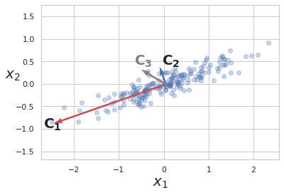
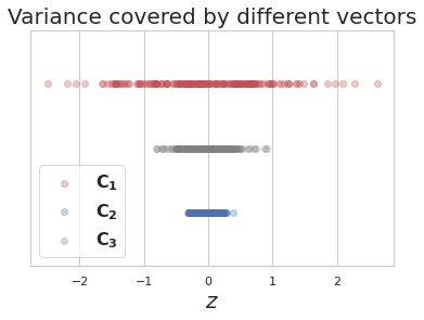
\(z\) represents projection of data points on a candidate vector.

Out of 3 candidate vectors to project data on, vector \(C_1\) captures most of the variance, hence it is the first PC and \(C_2\), which is orthogonal to it is the second PC

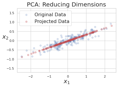
After applying PCA and choosing only first PC to reduce dimension of data.

Part 4: Chaining transformers

The preprocessing transformations are applied one after another on the input feature matrix.

It is important to apply exactly same transformation on training, evaluation and test set in the same order.

Failing to do so would lead to incorrect predictions from model due to distribution shift and hence incorrect performance evaluation.

si = SimpleImputer()
X_imputed = si.fit_transform(X)
ss =StandardScaler()
X_scaled = ss.fit_transform(X_imputed)

Class	Usage
Pipeline	Constructs a chain of multiple transformers to execute a fixed sequence of steps in data preprocessing and modelling.
FeatureUnion	Combines output from several transformer objects by creating a new transformer from them.

The sklearn.pipeline module provides utilities to build a composite estimator, as a chain of transformers and estimators.

There are two classes: (i) Pipeline and (ii) FeatureUnion.

`sklearn.pipeline.Pipeline`

Sequentially apply a list of transformers and estimators.

The purpose of the pipeline is to assemble several steps that can be cross-validated together while setting different parameters.

Intermediate steps of the pipeline must be ‘transformers’ that is, they must implement fit and transform methods.

The final estimator only needs to implement fit.

Pipeline()

Creating Pipelines

make_pipeline

It takes a list of ('estimatorName', estimator(...)) tuples.
The pipeline object exposes interface of the last step.

It takes a number of estimator objects only.

estimators = [
  ('simpleImputer', SimpleImputer()),
  ('standardScaler', StandardScaler()),
]
pipe = Pipeline(steps=estimators)

pipe = make_pipeline(SimpleImputer(),
                     StandardScaler())

Two ways to create a pipeline object.

estimators = [
  ('simpleImputer', SimpleImputer()),
  ('standardScaler', StandardScaler()),
]
pipe = Pipeline(steps=estimators)
pipe.fit_transform(X)

si = SimpleImputer()
X_imputed = si.fit_transform(X)
ss =StandardScaler()
X_scaled = ss.fit_transform(X_imputed)

Without pipeline:

With pipeline:

Accessing individual steps in Pipeline

estimators = [
  ('simpleImputer', SimpleImputer()),
  ('pca', PCA()),
  ('regressor', LinearRegression())
]
pipe = Pipeline(steps=estimators)

The second estimator can be accessed in following 4 ways:

pipe.named_steps.pca
pipe.steps[1]
pipe[1]
pipe['pca']

Total # steps: 3

SimpleImputer
PCA
LinearRegression

Accessing parameters of each step in Pipeline

Parameters of the estimators in the pipeline can be accessed using the <estimator>__<parameterName> syntax, note there are two underscores between <estimator> and <parameterName>

estimators = [
  ('simpleImputer', SimpleImputer()),
  ('pca', PCA()),
  ('regressor', LinearRegression())
]
pipe = Pipeline(steps=estimators)

pipe.set_params(pca__n_components = 2)

In above example n_components of PCA() step is set after the pipeline is created.

Performing grid search with pipeline

By using naming convention of nested parameters, grid search can implemented.

param_grid = dict(imputer=['passthrough', 
                           SimpleImputer(), 
                           KNNImputer()],
                  clf=[SVC(), LogisticRegression()],
                  clf__C=[0.1, 10, 100])
grid_search = GridSearchCV(pipe, param_grid=param_grid)

C is an inverse of regularization, lower its value stronger the regularization is.
In the example above clf__C provides a set of values for grid search.

Caching transformers

Transforming data is a computationally expensive step.
For grid search, transformers need not be applied for every parameter configuration. They can be applied only once, and the transformed data can reused.
This can be achieved by setting memory parameter of a pipeline object.
memory can take either location of a directory in string format or joblib.Memory object.

estimators = [
  ('simpleImputer', SimpleImputer()),
  ('pca', PCA(2)),
  ('regressor', LinearRegression())
]
pipe = Pipeline(steps=estimators, memory = '/path/to/cache/dir')

Combines multiple steps of end to end ML into single object such as missing value imputation, feature scaling and encoding, model training and cross validation.
Enables joint grid search over parameters of all the estimators in the pipeline.
Makes configuring and tuning end to end ML quick and easy.
Offers convenience, as a developer has to call fit() and predict() methods only on a Pipeline object (assuming last step in the pipeline is an estimator).
Reduces code duplication: With a Pipeline object, one doesn't have to repeat code for preprocessing and transforming the test data.

Advantages of pipeline

Concatenates results of multiple transformer objects.
Applies a list of transformer objects in parallel, and their outputs are concatenated side-by-side into a larger matrix.
FeatureUnion and Pipeline can be used to create complex transformers.

`sklearn.pipeline.FeatureUnion`

Combining Transformers and Pipelines

FeatureUnion() accepts a list of tuples.
Each tuple is of the format:
- ('estimatorName',estimator(...))

num_pipeline = Pipeline([('selector',ColumnTransformer([('select_first_4', 
                                                         'passthrough', 
                                                         slice(0,4))])),
                         ('imputer', SimpleImputer(strategy="median")),
                         ('std_scaler', StandardScaler()),
                        ])
cat_pipeline = ColumnTransformer([('label_binarizer', LabelBinarizer(),[4]),
                                  ])
full_pipeline = FeatureUnion(transformer_list=
                             [("num_pipeline", num_pipeline),
                              ("cat_pipeline", cat_pipeline),])

Visualizing Composite Transformers

from sklearn import set_config
set_config(display='diagram')   
# displays HTML representation in a jupyter context
full_pipeline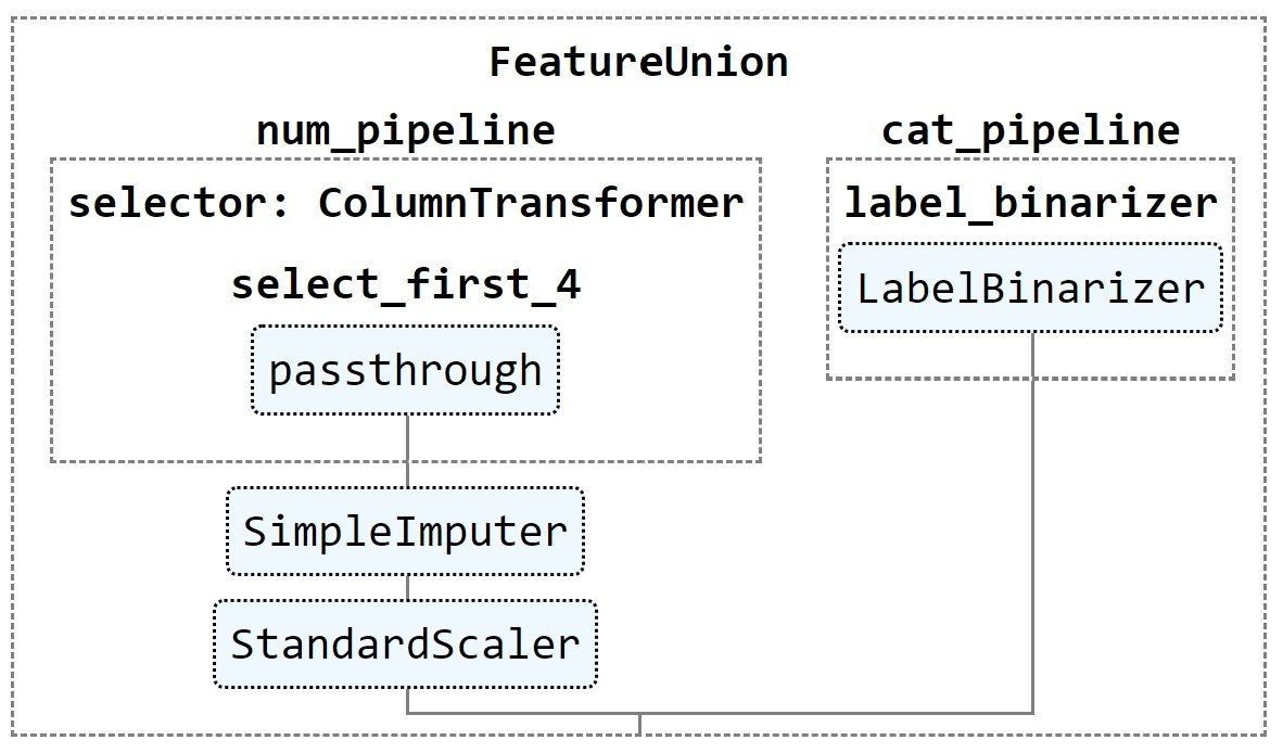

It creates the following visualization

That's it from data preprocessing.

Only way to master is to practice it with examples.

Read more about these methods in sklearn user guide on data transformation and documentation of different classes.