Support Vector Machines

Dr. Ashish Tendulkar

Machine Learning Practice

IIT Madras

In this week, we will study how to implement support vector machines for classification tasks with sklearn.

Support Vector Machines (SVM) are a set of supervised learning methods used for classification, regression and outliers detection.

Support Vector Machines

In sklearn, we have three methods to implement SVM.

SVC

NuSVC

LinearSVC

SVM constructs a hyper-plane or set of hyper-planes in a high or infinite dimensional space, which can be used for classification, regression or other tasks.

These are similar methods but, accept slightly different sets of parameters.

Implementation is based on libsvm.

Faster implementation of linear SVM classification with only linear kernel.

Implementation is based on liblinear.

shape \(\rightarrow\) (n_samples, n_features)

Training data

Array \(X\) : holding the training samples

Array \(y\) : holding the class labels (strings or integers)

shape \(\rightarrow\) (n_samples)

X = [[0, 0], [1, 1]]

y = [0,1]

How to implement SVC (C-Support Vector Classification)?

Step 1: Instantiate a SVC classifier estimator.

from sklearn.svm import SVC
SVC_classifier = SVC()

Step 2: Call fit method on SVC classifier object with training feature matrix and label vector as arguments.

# Model training with feature matrix X_train and 
# label vector or matrix y_train
SVC_classifier.fit(X_train, y_train)

How to perform regularization in SVC classifier?

C

Regularization parameter

SVC_classifier = SVC(C=1.0)

Default:

float value

strength of the regularization is inversely proportional to C
strictly positive
penalty is a squared l2 penalty

Note:

How to specify kernel type to be used in the algorithm ?

kernel

‘rbf’

SVC_classifier = SVC(kernel = 'rbf')

Default:

‘linear’

If kernel = poly , set degree (any integer value)
If kernel = callable is given it is used to pre-compute the kernel matrix from data matrices

‘poly’

‘sigmoid’

‘precomputed’

How to set kernel coefficient for 'rbf', 'poly' and 'sigmoid' kernels?

gamma

‘auto’

float value

value of gamma = \(\frac{1}{\text{number of features} ^*\text{X.Var()}}\)

value of gamma = \(\frac{1}{\text{number of features}}\)

‘scale’

SVC_classifier = SVC(gamma = 'scale')

Default:

If kernel = 'poly' or 'sigmoid' , set coef0 which is an independent term in kernel function (any integer value)

After the classifier is fit on the training data, there are few attributes which reveal the details of support vectors.

from sklearn.svm import SVC
SVC_classifier = SVC()
clf = SVC_classifier.fit(X_train, y_train)

#to view indices of the support vectors
clf.support_

#to view the support vectors
clf.support_vectors_

#to view the number of support vectors for each class
clf.n_support_

How to view support vectors?

How to implement NuSVC (\(\nu\)-Support Vector Classification)?

Step 1: Instantiate a NuSVC classifier estimator.

from sklearn.svm import NuSVC
NuSVC_classifier = NuSVC()

Step 2: Call fit method on NuSVC classifier object with training feature matrix and label vector as arguments.

# Model training with feature matrix X_train and 
# label vector or matrix y_train
NuSVC_classifier.fit(X_train, y_train)

\(\nu\) is an upper bound on the fraction of margin errors and and a lower bound of the fraction of support vectors.

What is the significance of \(\nu\) in NuSVC?

Value of \(\nu\) should \(\in (0,1]\)

Default:

\(\nu = 0.5\)

Instead of C in SVC, \(\nu\) is introduced in NuSVC to control the number of support vectors and margin errors.

Other parameters for NuSVC are same as that of SVC.

How to implement LinearSVC (Linear Support Vector Classification)?

Step 1: Instantiate a LinearSVC classifier estimator.

from sklearn.svm import LinearSVC
LinearSVC_classifier = LinearSVC()

Step 2: Call fit method on SVC classifier object with training feature matrix and label vector as arguments.

# Model training with feature matrix X_train and 
# label vector or matrix y_train
LinearSVC_classifier.fit(X_train, y_train)

Advantages of LinearSVC

It has more flexibility in the choice of penalties and loss functions since it is implemented in terms of liblinear.
Scales better to large numbers of samples.
Supports both dense and sparse input.

How to provide penalty in LinearSVC classifier?

LinearSVC_classifier = Linear_SVC(penalty = 'l2')

Default:

penalty

\(l2\) - adds a L2 penalty term

\(l1\) - adds a L1 penalty term

\(l1\) - leads to coef_ vectors that are sparse.

How to choose loss functions in LinearSVC classifier?

LinearSVC_classifier = Linear_SVC(loss = 'squared_hinge')

Default:

Combination not supported:

penalty='l1' and loss='hinge'

loss parameter

'hinge' - standard SVM loss

'squared_hinge' - square of the hinge loss

Some parameters in LinearSVC classifier

C

dual

fit_intercept

Regularization parameter

Select the algorithm to either solve the dual or primal optimization problem.
When n_samples >n_features, prefer dual=False.

To calculate the intercept for the model.

How to perform multi-class classification using SVM?

SVC and NuSVC implement the “one-versus-one” approach for multi-class classification.

LinearSVC implements “one-vs-the-rest” approach for multi-class classification.

multi_class

‘ovr’

‘crammer_singer’

decision_function_shape

‘ovo’

‘ovr’

Advantages of SVM

Effective in high dimensional spaces.
Effective in cases where number of dimensions is greater than the number of samples.
Uses a subset of training points in the decision function (called support vectors), so it is also memory efficient.
Versatile: different Kernel Functions can be specified for the decision function.

Disadvantages of SVM

SVMs do not directly provide probability estimates, these are calculated using an expensive five-fold cross-validation.
Avoid over-fitting in choosing Kernel functions if the number of features is much greater than the number of samples.

Appendix

Classification

SVC

Class: \(\colorbox{lightgrey}{sklearn.svm.SVC}\)

Some Parameters:

C (float, default=1.0): It is a regularization parameter. The strength of the regularization is inversely proportional to C. It should always be positive.
kernel (‘linear’, ‘poly’, ‘rbf’, ‘sigmoid’, ‘precomputed’, default=’rbf’):Specifies the kernel type to be used in the algorithm.
degree (int, default=3): Degree of the polynomial kernel function (‘poly’). Ignored for all other kernels.

SVC

gamma(‘scale’, ‘auto’ or float, default=’scale’): Kernel coefficient for ‘rbf’ (Gaussian), ‘poly’(Polynomial) and ‘sigmoid’.
cache_size(float, default=200): It specifies the size of the kernel cache (in MB).
max_iter(int, default=-1): It represents hard limit on iterations within solver, or -1 for no limit.
random_state(int, default=None): Controls the pseudo random number generation for shuffling the data for probability estimates.

Some Parameters: (continued...)

NuSVC

Class: \(\colorbox{lightgrey}{sklearn.svm.NuSVC}\)

Some parameters:

nu(float, default=0.5): An upper bound on the fraction of margin errors and a lower bound of the fraction of support vectors. It should be in the interval (0, 1].
kernel(‘linear’, ‘poly’, ‘rbf’, ‘sigmoid’, ‘precomputed’, default=’rbf’)

Specifies the kernel type to be used in the algorithm.
degree (int, default=3): Degree of the polynomial kernel function (‘poly’). Ignored for all other kernels.

NuSVC

gamma(‘scale’, ‘auto’ or float, default=’scale’): Kernel coefficient for ‘rbf’, ‘poly’(Polynomial) and ‘sigmoid’.
cache_size(float, default=200): It specifies the size of the kernel cache (in MB).
max_iter(int, default=-1): It represents hard limit on iterations within solver, or -1 for no limit.
random_state(int, default=None): Controls the pseudo random number generation for shuffling the data for probability estimates.

Some Parameters: (continued...)

LinearSVC

Class: \(\colorbox{lightgrey}{sklearn.svm.LinearSVC}\)

Some parameters:

penalty(‘l1’, ‘l2’, default=’l2’): It specifies the norm used in the penalization. The ‘l2’ penalty is the standard used in SVC. The ‘l1’ leads to coef_ vectors that are sparse.
loss(‘hinge’, ‘squared_hinge’, default=’squared_hinge’): It specifies the loss function.
C (float, default=1.0): It is a regularization parameter. The strength of the regularization is inversely proportional to C. It should always be positive.

LinearSVC

Some parameters: Continued...

fit_intercept(bool, default=True): Whether to calculate the intercept for this model. If set to false, no intercept will be used in calculations (i.e. data is expected to be already centered).
dual(bool, default=True): Select the algorithm to either solve the dual or primal optimization problem. Prefer dual=False when .
max_iter(int, default=1000): It represents the maximum number of iterations to be run.

\color{red}{n_{samples} > n_{features}}

Plot different SVM classifiers in the iris dataset

The below example shows how to plot the decision surface for four SVM classifiers with different kernels.

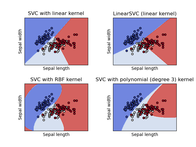
We are considering only the first two features of the iris dataset.

Sepal Length

Sepal width

Classification

They are capable of performing binary and multi-class classification on a dataset.

LinearSVC does not accept parameter kernel, as this is assumed to be linear. It also lacks some of the attributes of SVC and NuSVC, like support.

SVC and NuSVC are similar methods, but accept slightly different sets of parameters and have different mathematical formulations. On the other hand, LinearSVC is another (faster) implementation of Support Vector Classification for the case of a linear kernel.

SVC, NuSVC and LinearSVC take as input two arrays:

- an array x of shape (n_samples, n_features) holding the training samples.

- an array y of class labels (strings or integers), of shape (n_samples).

Examples

1. SVM: Maximum Margin Separating hyperplane

Below is the plot for maximum margin separating hyperplane within a two-class separable dataset using a Support Vector Machine classifier with linear kernel.

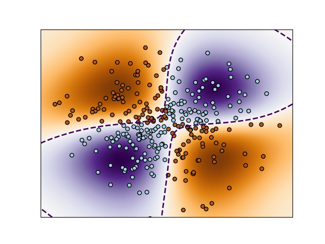
2. Non-linear SVM

Binary classification with RBF kernel using non-linear SVC.

We are predicting the XOR of the inputs.

Illustration of decision function learnt by SVC

3. SVM-Anova:

SVM with univariate feature selection

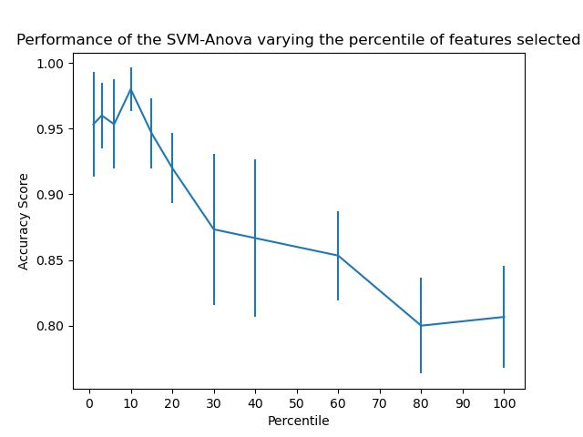
It shows how to perform univariate feature selection before running a SVC (support vector classifier) to improve the classification scores.

Take 4 features from the iris dataset.

Add another 36 non-informative features.

This model achieves the best performance when we select around 10% of features.

Classification

1. Multi-class classification

2. Scores and Probabilities

3. Unbalanced problems

Multi-class classification

There are two approaches for multi-class classification:

One vs one
One vs rest

SVC and NuSVC implement the “one-vs-one” approach for multi-class classification. In total, n_classes * (n_classes - 1) / 2 classifiers are constructed and each one trains data from two classes.
To provide a consistent interface with other classifiers, the decision_function_shape option allows to monotonically transform the results of the “one-vs-one” classifiers to a “one-vs-rest” decision function of shape (n_samples, n_classes).
LinearSVC implements “one-vs-rest” multi-class strategy, thus training n_classes models.

Scores and Probabilities

Unbalanced problems

In problems, where it is desired to give more importance to certain classes or certain individual samples, these parameters can be used:

class_weight

sample_weight

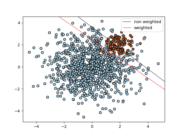
The example illustrates the decision boundary of an unbalanced problem, with and without weight correction.

SVM: Separating hyperplane for unbalanced classes

The figure below illustrates the effect of sample weighting on the decision boundary. The size of the circles is proportional to the sample weights:

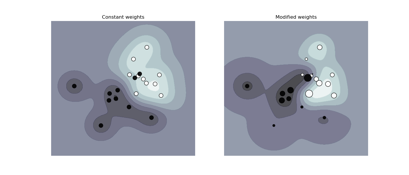
The sample weighing rescales the parameter \(c\), which means that the classifier puts more emphasis on getting these points right.

SVM: Weighted samples

Regression

The method of SVC can be extended to solve regression problems. This method is called Support Vector Regression.

The model produced by Support Vector Regression depends only on a subset of the training data, because the cost function ignores samples whose prediction is close to their target.

There are three different implementations of Support Vector Regression: SVR, NuSVR and LinearSVR.

SVR

Class: \(\colorbox{lightgrey}{sklearn.svm.SVR}\)

Some Parameters:

C (float, default=1.0): It is a regularization parameter. The strength of the regularization is inversely proportional to C. It should always be positive.
kernel (‘linear’, ‘poly’, ‘rbf’, ‘sigmoid’, ‘precomputed’, default=’rbf’):

Specifies the kernel type to be used in the algorithm.
degree (int, default=3): Degree of the polynomial kernel function (‘poly’). Ignored for all other kernels.
gamma(‘scale’, ‘auto’ or float, default=’scale’): Kernel coefficient for ‘rbf’ (Gaussian), ‘poly’(Polynomial) and ‘sigmoid’.

SVR

epsilon(float, default=0.1): Epsilon in the epsilon-SVR model. It specifies the epsilon-tube within which no penalty is associated in the training loss function with points predicted within a distance epsilon from the actual value.
cache_size(float, default=200): It specifies the size of the kernel cache (in MB).
max_iter(int, default=-1): It represents hard limit on iterations within solver, or -1 for no limit.
random_state(int, default=None): Controls the pseudo random number generation for shuffling the data for probability estimates.

Some Parameters: (continued...)

NuSVR

Class: \(\colorbox{lightgrey}{sklearn.svm.NuSVR}\)

Some parameters:

nu(float, default=0.5): It represents an upper bound on the fraction of training errors and a lower bound of the fraction of support vectors. It should be in the interval (0, 1]. By default, 0.5 will be taken.
C(float, default=1.0): A penalty parameter of the error term.
kernel(‘linear’, ‘poly’, ‘rbf’, ‘sigmoid’, ‘precomputed’, default=’rbf’):

Specifies the kernel type to be used in the algorithm.

NuSVR

degree (int, default=3): Degree of the polynomial kernel function (‘poly’). Ignored for all other kernels.
gamma(‘scale’, ‘auto’ or float, default=’scale’): Kernel coefficient for ‘rbf’ (Gaussian), ‘poly’(Polynomial) and ‘sigmoid’.
cache_size(float, default=200): It specifies the size of the kernel cache (in MB).
max_iter(int, default=-1): It represents hard limit on iterations within solver, or -1 for no limit.

Some Parameters: (continued...)

LinearSVR

Class: \(\colorbox{lightgrey}{sklearn.svm.LinearSVR}\)

Some parameters:

epsilon(float, default=0.0): Epsilon parameter in the epsilon-insensitive loss function. Note that the value of this parameter depends on the scale of the target variable y.
loss(epsilon_insensitive’, ‘squared_epsilon_insensitive’, default=’epsilon_insensitive’) : It specifies the loss function. The epsilon-insensitive loss (standard SVR) is the L1 loss, while the squared epsilon-insensitive loss is the L2 loss.
C (float, default=1.0): It is a regularization parameter. The strength of the regularization is inversely proportional to C. It should always be positive.

LinearSVR

Some parameters: Continued...

fit_intercept(bool, default=True): Whether to calculate the intercept for this model. If set to false, no intercept will be used in calculations (i.e. data is expected to be already centered).
dual(bool, default=True): Select the algorithm to either solve the dual or primal optimization problem. Prefer dual=False when n_samples > n_features.
max_iter(int, default=1000): It represents the maximum number of iterations to be run.

Density estimation, Novelty detection

The class OneClassSVM implements a One-Class SVM which we use in outlier detection. Outlier detection and novelty detection are both used for anomaly detection

Novelty detection:

The training data is not polluted by outliers and we are interested in detecting whether a new observation is an outlier. In this context an outlier is also called a novelty.

Outlier detection:

The training data contains outliers which are defined as observations that are far from the others. Outlier detection estimators thus try to fit the regions where the training data is the most concentrated, ignoring the deviant observations.

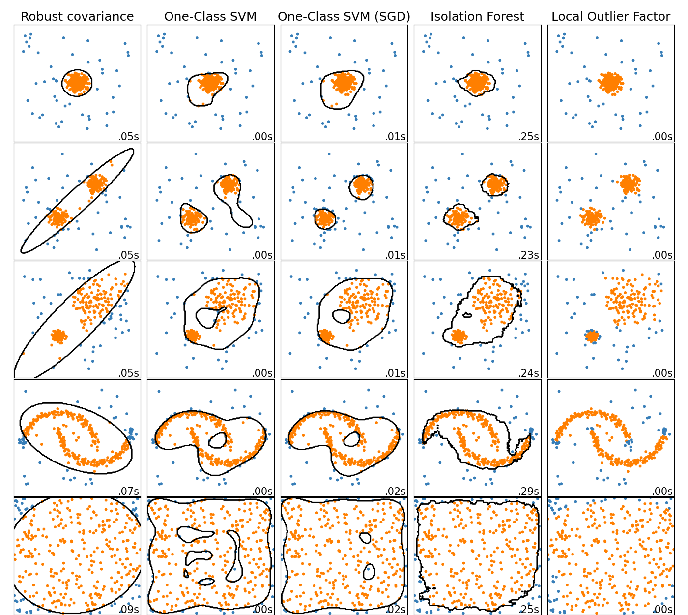
Here, Local Outlier Factor (LOF) does not show a decision boundary in black.

An overview of outlier detection method

This shows a comparison of the outlier detection algorithms in scikit-learn.

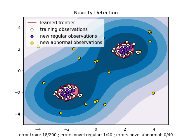
An example using a one-class SVM for novelty detection.

One-class SVM is an unsupervised algorithm that learns a decision function for novelty detection: classifying new data as similar or different to the training set

Complexity

The computation and storage requirements increase rapidly with the number of training vectors in SVM.
The core of an SVM is a quadratic programming problem (QP).
The QP solver used by the libsvm-based implementation scales between \(O(n_{features}\times n^2_{samples})\) and \(O(n_{features}\times n^3_{samples})\) depending on how efficiently the libsvm cache is used in practice.

Note: If the data is very sparse \(n_{features}\) should be replaced by the average number of non-zero features in a sample vector.

Kernel functions

The kernel function can be any of the following:

linear: \(\langle x, x' \rangle\)

polynomial: \((\gamma\langle x, x' \rangle+r)^d\)

rbf: \(\exp (-\gamma\lVert x-x'\rVert^2)\)

- \(d\) is specified by parameter

degree

- \(r\) is specified by parameter

coef\(\theta\)

- \(\gamma\) is specified by parameter

sigmoid: \(\tanh(\gamma \langle x, x' \rangle)+r\)

gamma

- \(\gamma>0\)

- \(r\) is specified by parameter

coef\(\theta\)

Parameters of the RBF Kernel

The parameters that must be considered while training an SVM with the Radial Basis Function (RBF) kernel are: and .

\(c\)

gamma

A low value of \(c\) makes the decision surface smooth.

A high value of \(c\) aims at classifying all training examples correctly.

The larger gamma is, the closer other examples must be to be affected.

Custom Kernels

One can define their own kernels by either giving the kernel as a python function or by precomputing the Gram matrix.

Using Python function as Kernels

Using the Gram matrix

by passing a function to the parameter.

kernel

arguments

- (n_samples_1, n_features)

- (n_samples_2, n_features)

return

- (n_samples_1, n_samples_2)

by passing a pre-computed kernels by

kernel='precomputed'

Classifiers with custom kernels behave the same way as any other classifiers with few exceptions:

- Field is now empty.

support_vectors_

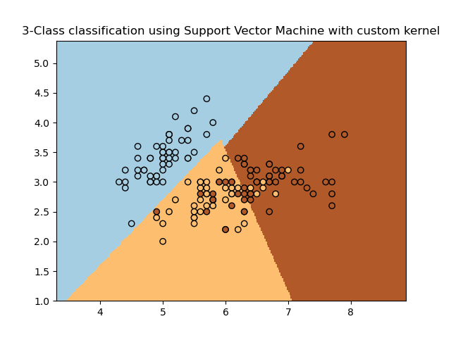
It will plot the decision surface and the support vectors.

Example: SVM with custom kernel

Mathematical Formulation

Intuitively, a good separation is achieved by the hyper-plane that has the largest distance to the nearest training data points of any class (so-called functional margin), since in general the larger the margin the lower the generalization error of the classifier.

A support vector machine constructs a hyper-plane or set of hyper-planes in a high or infinite dimensional space, which can be used for classification, regression or other tasks.

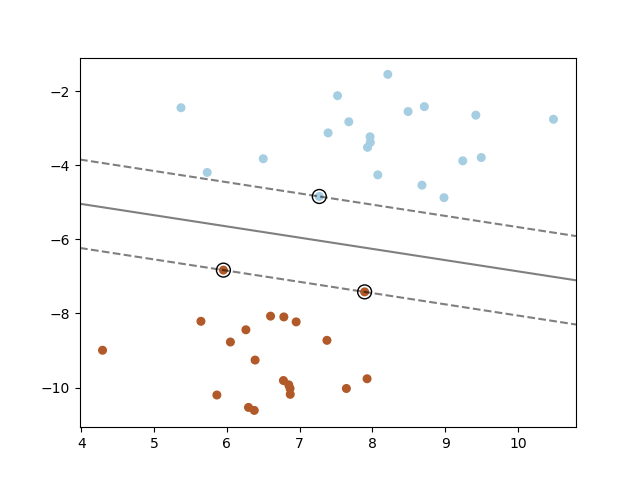
The figure below shows the decision function for a linearly separable problem, with three samples on the margin boundaries, called " support vectors " :

Note: When the problem isn’t linearly separable, the support vectors are the samples within the margin boundaries.

SVC

Primal Problem:

\(\min \dfrac{1}{2}w^Tw+c\sum\limits_{i=1}^{n}\zeta_i\)

subject to \(~~~~~~~~~~~~y_i(w^T\phi(x_i)+b)\geq 1-\zeta_i, ~~~~~~~~\zeta_i\geq 0, i: 1,\cdots, n.\)

Given training vectors \(x_i\in \mathbb{R}^p\), \(i=1, \cdots, n\), in two classes, and a vector \(y \in \{-1, 1\}^n\), our goal is to find \(w \in \mathbb{R}^p\) and \(b \in \mathbb{R}\) such that the prediction given by \(sign(w^T\phi(x)+b)\) is correct for most samples.

Intuitively, we’re trying to maximize the margin (by minimizing \(\Vert w \Vert^2 = w^Tw\)).

Ideally, \(y_i(w^T\phi(x_i)+b)\) would be greater than equal to 1 for all samples, which indicates a perfect prediction.

We allow some samples to be at a distance \(\zeta_i\) from their correct margin boundary since the problems are usually not always perfectly separable.

\(c\) : the penalty term, controls the strength of the penalty.

Dual Problem:

\(\min\limits_{\alpha}\dfrac{1}{2}\alpha^TQ\alpha - e^T\alpha\)

subject to \(~~~~~~~~~~~~~~~y^T\alpha = 0, ~~~~~~~~~~~~~~~~~~~~~~~~~~~~~\)

\(0\leq \alpha_i\leq c, i = 1, \cdots, n.\)

\(e\) is the vector of all ones.

\([Q]_{n\times n}\) is a positive semi - definite matrix.

\(Q_{ij} \equiv y_iy_j K(x_i, x_j)\) is the kernel, where \(K(x_i, x_j) = \phi(x_i)^T\phi(x_j)\).

\(\alpha_i\) - dual coefficients

Once the optimization problem is solved, the output of decision_function for a given sample \(x\) becomes:

\(\sum\limits_{i\in SV}y_i\alpha_iK(x_i, x)+b\)

These parameters can be accessed through the attributes:

\(\nearrow\)

\(\longrightarrow\)

\(\searrow\)

- dual_coef_

- support_vectors_

- intercept_

: holds the product \((y_i \alpha_i^*)\)

: holds the support vectors

: holds the independent term \(b\) .

Linear SVC

The primal problem can be formulated as

\(\min\limits_{w, b}\dfrac{1}{2}w^Tw+c\sum\limits_{i=1}\max(0, 1-y_i(w^T\phi(x_i)+b))\)

We make use of the hinge loss (a loss function used for training classifiers).

directly optimized by LinearSVC.

kernel trick cannot be applied.

only the linear kernel is supported by LinearSVC.

NuSVC

\(\nu\) - SVC and \(C\) - SVC are mathematically equivalent.

Instead of \(C\), introduce a new parameter \(\nu\).

\(\nu\) controls the number of support vectors and margin errors.

\(\color{blue}{\Huge \curvearrowright}\)

A margin error corresponds to a sample that lies on the wrong side of its margin boundary is either misclassified, or is correctly classified but does not lie beyond the margin.

SVR

Given training vectors \(x_i\in \mathbb{R}^p, i: 1,\cdots, n\), and a vector \(y\in \mathbb{R}^n\), \(\epsilon\)-SVR solves the following primal problem:

\(\min\limits_{w, b, \zeta, \zeta*}\dfrac{1}{2}w^Tw+C\sum\limits_{i=1}^{n}(\zeta_i+\zeta_i^*)\)

subject to \(~~~~~~~~~~~~y_i-w^T\phi(x_i)-b\leq \epsilon +\zeta_i \)

\(w^T\phi(x_i)+b-y_i\leq \epsilon +\zeta_i^*\)

\(\zeta_i, \zeta_i^*\geq 0, i: 1, \cdots, n\)

Primal problem

Dual Problem

\(\min\limits_{\alpha, \alpha^*}\dfrac{1}{2}(\alpha-\alpha^*)^TQ(\alpha-\alpha^*)+\epsilon e^T(\alpha+\alpha^*)-y^T(\alpha-\alpha^*)\)

subject to \(~~~~~~~~~~~~~~~~~~~e^T(\alpha-\alpha^*) = 0\)

\(0\leq \alpha_i, \alpha_i^*\leq C, i=1, \cdots, n\)

Here, we are penalizing samples whose prediction is at least \(\epsilon\) away from their true target.

Dual Problem

\(\min\limits_{\alpha, \alpha^*}\dfrac{1}{2}(\alpha-\alpha^*)^TQ(\alpha-\alpha^*)+\epsilon e^T(\alpha+\alpha^*)-y^T(\alpha-\alpha^*)\)

subject to \(~~~~~~~~~~~~~~~~~~~e^T(\alpha-\alpha^*) = 0\)

\(0\leq \alpha_i, \alpha_i^*\leq C, i=1, \cdots, n\)

\(e\) is the vector of all ones.

\([Q]_{n\times n}\) is a positive semi - definite matrix.

\(Q_{ij}\equiv K(x_i, x_j) = \phi(x_i)^T\phi(x_j)\) is the kernel.

Here training vectors are implicitly mapped into a higher (maybe infinite) dimensional space by the function \(\phi\).

The prediction is:

\(\sum\limits_{i \in SV}(\alpha_i - \alpha_i^*)K(x_i, x)+b\)

These parameters can be accessed through the attributes:

\(\nearrow\)

\(\longrightarrow\)

\(\searrow\)

- dual_coef_

: holds the difference \((\alpha_i - \alpha_i^*)\)

- support_vectors_

: holds the support vectors

- intercept_

: holds the independent term \(b\) .

Linear SVR

Primal problem:

\(\min\limits_{w, b}\dfrac{1}{2}w^Tw+C\sum\limits_{i=1}\max(0, \mid y_i-(w^T\phi(x_i)+b))\mid-\epsilon)\)

Here, we make use of the epsilon-insensitive loss, i.e., we ignore errors of less than \(\epsilon\).

This form is directly optimized by LinearSVR.

Implementation details

To handle all computations, we use the libraries libsvm and liblinear.

Libsvm

It is an integrated software for support vector classification, (C-SVC, nu-SVC), regression (epsilon-SVR, nu-SVR) and distribution estimation (one-class SVM).

It supports multi-class classification.

It's main features include:

- Different SVM formulations

- Efficient multi-class classification

- Cross validation for model selection

- Probability estimates

- Various kernels (including precomputed kernel matrix)

-GUI demonstrating SVM classification and regression

- Automatic model selection which can generate contour cross validation accuracy.

Liblinear

A library for large linear classification.

It's main feature includes:

- Multi-class classification: 1) one-vs-the rest, 2) Crammer & Singer

- Cross validation for model evaluation.

- Automatic parameter selection

- Probability estimates (logistic regression only)