Models of Regression
Dr. Ashish Tendulkar
Machine Learning Techniques
IIT Madras
Regression
It is a supervised learning problem where the output label is a real number.

Two types of regression
Single label regression
Multi label regression
Single output label: \(y \in \mathbf{R}\)
Multiple output labels - total labels \(k\): \( \mathbf{y} \in \mathbf{R}^k \)
e.g. Predict temperature for tomorrow based on weather features of past days
e.g. Predict temperature for next 5 days based on weather features of past days
What will be covered in this module?
- Linear regression
- Polynomial regression
- Regularization
All concepts will be discussed for single label regression problem set up.
In the end, we will extend them to multi-label regression problem set up.
Linear Regression
It is a machine learning algorithm that predicts real valued output label based on linear combination of input features.
- Input: Feature vector \(\mathbf{x}_{m×1}\).
- Label: \(y \in \mathbb{R}\), which is a scalar. (Single label set up)
Part I: Linear Regression
Data
Data
A set of \(n\) ordered pairs of a feature vector, \(\mathbf{x}\) and a label \(y\) representing examples. We denote it by \(D\):
\( D = \left\{ (\mathbf{X}, \mathbf{y})\right\} = \left\{ (\mathbf{x}^{(i)}, y^{(i)})\right\}_{i=1}^{n} \)
Features
\(\mathbf{X}\) is a feature matrix corresponding to \(n\) training examples, each represented with \(m\) features and has shape \(n \times m\). In this matrix, each feature vector is transposed and represented as a row.
Feature vector for \(i\)-th training example \(\mathbf{x}^{(i)}\) can be obtained by \(\mathbf{X}[i]\)
Labels
For single label problem, \(\mathbf{y}\) is a label vector of shape \(n \times 1\).
The \(i\)-th entry in this vector, \(\mathbf{y}[i]\) gives label for \(i\)-th example, which is denoted by \(y^{(i)} \in \mathbb{R}\)
Data: Example
No. of
Floors
Sample House Pricing data is presented below.
Area
Age
House 1
House 2
House 3
House 4
Features (m=3)
Examples (n=4)
\( D = \left\{ (\mathbf{X}, \mathbf{y})\right\} = \left\{ (\mathbf{x}^{(i)}, y^{(i)})\right\}_{i=1}^{n} \)
Data: Example
No. of
Floors
It has three features: area in square feet, no. of floors and age in years, for 4 houses.
Area
Age
House 1
House 2
House 3
House 4
Data: Example
No. of
Floors
Here number of samples \(n\) is 4 and number of features \(m\) is 3
Area
Age
House 1
House 2
House 3
House 4
Area
House Pricing data, first feature only
House 1
House 2
House 3
House 4
Data: Example
House Pricing data, one sample only
House 1
No. of Floors
Area
Age
Data: Example
House Pricing data, one sample only
House 1
No. of
Floors
Area
Age
Data: Example
Data: Example
Price
House Pricing data, labels (price in Rs.)
House 1
House 2
House 3
House 4
Data: Example
Price
House 1
House 2
House 3
House 4
No. of
Floors
Area
Age
\( D = \left\{ (\mathbf{X}_{4 \times 3}, \mathbf{y}_{4\times 1})\right\} = \left\{ (\mathbf{x}^{(i)}, y^{(i)})\right\}_{i=1}^{4} \)
Model
Model
- Each feature \(x_j\) has a corresponding weight \(w_j\).
- Let's introduce a dummy feature \(x_0 = 1\) for weight \(w_0\):
Label \(y\) is computed as a linear combination of features \(x_1,x_2,...,x_m\):
\(y = \color{red}{w_0} \color{black}+ \color{red}{w_1} \color{black}{x_1} + \color{red}{w_2} \color{black}{x_2} + \ldots + \color{red}{w_m} \color{black}{x_m}\)
\(y = \color{red}{w_0} \color{blue}{x_0} \color{black}+ \color{red}{w_1} \color{black}{x_1} + \ldots + \color{red}{w_m} \color{black}{x_m} \)
\(y = \sum\limits_{i=0}^{m} \color{red}{w_i} \color{black}{x_i}\)
It can be written compactly as
Here \(\color{red}{w_0,w_1, w_2, \ldots, w_m}\color{black}\) are weights
How does the model look like?
Take a simple model with a single feature \(x_1\):
\(y = \color{red}{w_0} \color{black}+ \color{red}{w_1} \color{black}{x_1} \)
# model parameters (2): \( \color{red}{w_0} \color{black}, \color{red}{w_1} \)
Each new combination of \( \color{red}{w_0} \color{black}, \color{red}{w_1} \) leads to a new model.
Total # of possible models = infinite
| # Features (m) | Model | Geometry | # Params (# w) |
|---|---|---|---|
| line | 2 | ||
| plane | 3 | ||
| hyperplane in (m +1)-D |
Model: geometry and # parameters depends on # features
\(m+1\)
\(y = \sum\limits_{i=0}^{m} \color{red}{w_i} \color{black}{x_i}\)
\(y = \color{red}{w_0} \color{black}+ \color{red}{w_1} \color{black}{x_1} \)
\(y = \color{red}{w_0} \color{black}+ \color{red}{w_1} \color{black}{x_1} + \color{red}{w_2} \color{black}{x_2} \)
\( \ge 3 \)
\(1\)
\(2\)
Model: Vectorized Form
\(y = \sum\limits_{j=0}^{m} \color{red}{w_j} \color{black}{x_j}\) = \( \color{red}{\mathbf{w}^T}\color{black} \mathbf{x}\)
All weights \(w_0, w_1, \ldots, w_m\) can be arranged in a vector \(\mathbf{w}\) with shape \((m+1) \times 1\)
Solve vector matrix product and verify it corresponds to the linear combination of features.
Exercise: Check \( \color{red}\mathbf{w}^T\color{black}\mathbf{x} = \sum \color{red}w_j \color{black} x_j\)
The features for an \(i\)-th example can also be represented as a feature vector \(\mathbf{x}^{(i)}\). Note that we add a special feature \(x_0\).
Setting \( x_0 = 1 \)
Exercise: Check \( \color{red}\mathbf{w}^T\color{black}\mathbf{x} = \sum \color{red}w_j \color{black} x_j\)
Let's multiply these vectors to obtain \(y^{(i)}\):
Exercise: Check \( \color{red}\mathbf{w}^T\color{black}\mathbf{x} = \sum \color{red}w_j \color{black} x_j\)
\(y^{(i)} = \sum\limits_{j=0}^{m} \color{red}{w_j} \color{black}{{x_j}^{(i)}}\)
\(y^{(i)} = \color{red}{w_0} \color{black}\times 1 + \color{red}{w_1} \color{black}\times x_1^{(i)} + \color{black} \ldots + \color{red}{w_m} \color{black} \times x_m^{(i)}\)
\(y^{(i)} = \color{red}{w_0} \color{blue}{x_0} \color{black} + \color{red}{w_1} \color{black} x_1^{(i)} + \color{red}{w_2} \color{black} x_2^{(i)} + \ldots + \color{red}{w_m} \color{black} x_m^{(i)}\)
Exercise: Check \( \color{red}\mathbf{w}^T\color{black}\mathbf{x} = \sum \color{red}w_j \color{black} x_j\)
A weight vector \(\mathbf{w}\) with shape \(\left(m+1 \right) \times 1\).
Vectorized implementation: Multiple Examples
A feature matrix \(\mathbf{X}\) has shape \((n, m+1)\) containing features for \(n\) examples.
The label vector \(\widehat{\mathbf{y}}\) containing labels for all the \(n\) examples can be computed as follows:
Model Inference
def predict(X, w):
  # Make sure features and weights have compatible shape.
  # Check to make sure that the shapes are compatible.
  assert X.shape[-1]==w.shape[0], "X and w don't have compatible dimensions"

  y = X @ w
  return y
Implement the model inference in vectorized form:
\(\mathbf{y} = \color{black}{\mathbf{X}}\color{red} \mathbf{w} \)
Choosing best-fit model
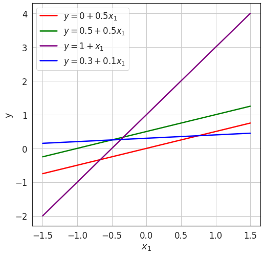
- Let's choose a simple model for exploring this question:
- As we vary \((\color{red}w_0 \color{black}, \color{red} w_1 \color{black} )\), we get a new model.
\(y = \color{red}{w_0}\color{black}+\color{red}{w_1} \color{black}{x_1}\)
Evaluate data fitment of model
- We need a measure of fitment or mis-fitment.
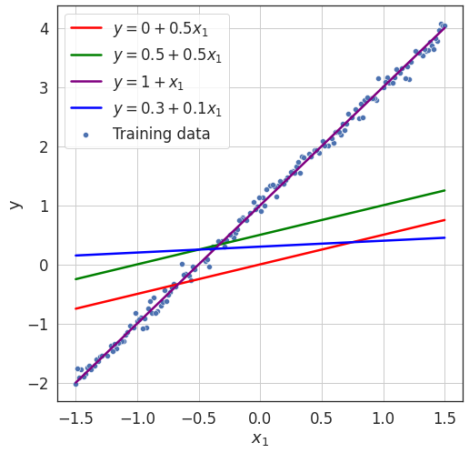
- Which one fits the training data better than all other models?
Loss or error function
Loss Function
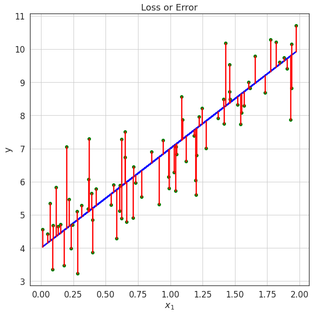
Loss Function: Sum of Squared Error (SSE)
SSE is the sum of square of difference between actual and predicted labels for each training point.
- The error \(e^{(i)}\) is non-negative or \(e^{(i)} \geq 0\).
- \(e^{(i)} = 0\), whenever the actual label and the predicted label are identical.
Error at \(i\)-th training point
Loss Function: SSE
The total loss \(J(\mathbf{w})\) is sum of errors at each training point:
We divide this by \(\dfrac{1}{2}\) for mathematical convenience in later use:
The loss is dependent on the value of \(\mathbf{w}\) - as these values change, we get a new model, which will result in different prediction and hence different error at each training point.
SSE vectorization for efficient computation
Recall, \(\hat\mathbf{y}= \mathbf{X} \mathbf{w} \)
\(= \frac{1}{2} \left( \color{blue}{{\mathbf{X} \mathbf{w}}} \color{black}-\mathbf{y} \right)^T \left( \color{blue}{{\mathbf{X} \mathbf{w}}} \color{black}-\mathbf{y} \right) \)
def loss(features, labels, weights):

  # Compute error vector
  e =  predict(features, weights) - labels

  # Compute loss
  loss = (1/2) * (np.transpose(e) @ e)

  return loss
Loss function visualization
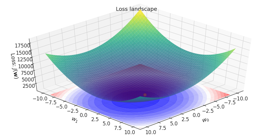
\( h_\mathbf{w}(\mathbf{x}): y = \color{red} w_0\color{black}+ \color{red}w_1 \color{black}x_1\)
Model
Loss (SSE)
Duality of loss and model spaces
How do we find the model with the least loss or error?
Optimization
Optimization
Key calculation is the derivative of loss function \(J(\mathbf{w})\) with respect to \(\mathbf{w}\).
Let's look at a couple of useful identities for this:
\(\dfrac{\partial}{\partial \mathbf{w}} \left( \mathbf{w} \mathbf{x} \right) = \dfrac{\partial}{\partial \mathbf{w}} \left( \mathbf{x}^T \mathbf{w}\right) = \dfrac{\partial}{\partial \mathbf{w}} \left( \mathbf{w}^T \mathbf{x} \right) = \mathbf{x} \)
Derivative of linear function:
Derivative of quadratic function:
Similar to \(\dfrac{d}{dw} (xw) = x\)
Similar to \(\dfrac{d}{dw} (xw^2) = 2xw\)
Computing gradient of loss function
Computing gradient of loss function
How to obtain \(\mathbf{w}\) ?
- Normal equation
- Gradient descent
Set the partial derivative to 0 and solve with analytical method to obtain the weight vector
Iteratively change the weights based on the partial derivative of the loss function until convergence (Iterative optimization)
Normal Equation
Let's set \(\dfrac{\partial J(\mathbf{w})}{\partial \mathbf{w}}\) to 0 and solve for \(\mathbf{w}\):
Recall \(\dfrac{\partial J(\mathbf{w})}{\partial \mathbf{w}} = \mathbf{X}^T \mathbf{X} \mathbf{w} - \mathbf{X}^T \mathbf{y} \)
Gradient Descent: Non Vectorized
- Randomly initialize the weight vector \(\mathbf{w}\). One possible initialization can be: \(w_0 = 0, w_1 = 0, \ldots, w_m=0\).
Gradient Descent: Non Vectorized
- Iterate until convergence:
-
Calculate gradient of loss function w.r.t. the weights \(w_0\), \(w_1\) .... \(w_m\), which are \(\dfrac{\partial J(\mathbf{w})}{\partial w_0}\), \(\dfrac{\partial J(\mathbf{w})}{\partial w_1}\) .... \(\dfrac{\partial J(\mathbf{w})}{\partial w_m}\) respectively.
-
Gradient Descent: Non Vectorized
Gradient Descent: Non Vectorized
- Calculate updated parameters:
Here \(\alpha\) is learning rate.
Gradient Descent: Non Vectorized
- Update parameters simultaneously:
After this step, we have a new weight vector.
Gradient Descent: Non Vectorized
- Note that the weights are updated to their new values simultaneously in the last step of GD .
- Until then the old values are used for predicting labels of examples while calculating the parameter updates.
Gradient Descent: Vectorized
This vectorized implementation will make sure that all the parameters are updated in one go.
Gradient Descent Visualization
\( h_\mathbf{w}(\mathbf{x}): y = \color{red} w_0\color{black}+ \color{red}w_1 \color{black}x_1\)
Model
Loss (SSE)
Gradient Descent: Salient Features
-
GD is a very generic optimization algorithm that can be used for learning weight vectors of most of the ML models.
-
GD obtains optimal weight vector by making small changes to their values in each iteration proportional to the gradient of the loss function.
-
Once GD reaches the minima of the loss function, we obtain the optimal weights corresponding to the minima.
Gradient Descent Convergence
-
The weight vector changes by a very small margin in successive iterations or in last few iterations.
-
After completing a fixed number of iterations.
Gradient Descent: Practical considereations
1. How do we set the learning rate \(\alpha\) ?
2. How do we decide the number of iterations?
Fixing learning rate \( \alpha \)
Try different values of \(\alpha\): \( \{0.0001, 0.001, 0.01, 0.1, 1 \} \)

Top one, with \(\alpha = 0.0001\) takes longer to reach optimal point, compared with \(\alpha = 0.001\)
Visualization based diagnosis is not possible for real-word problems with more features, learning curves are our best friends in general case.
Fixing \(\alpha\): Diagnosis based on learning curves
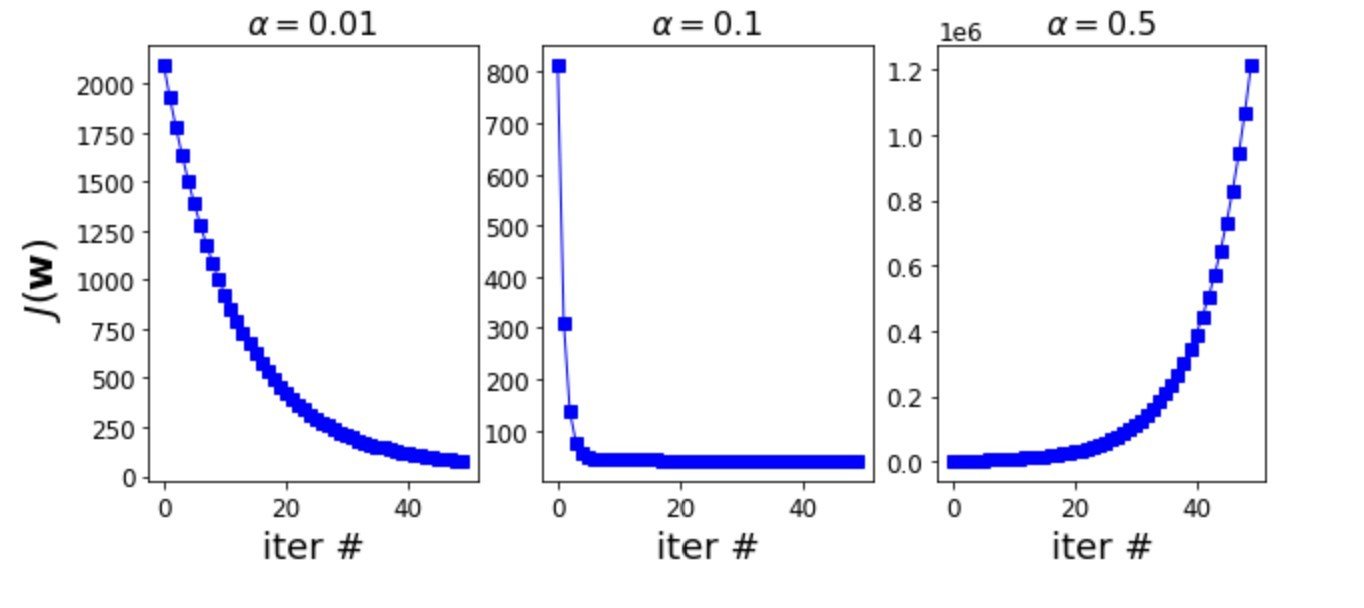
- After first 50 iterations, \(\alpha=0.1\)(middle one) has the lowest loss. Loss decreases rapidly.
- The loss for \(\alpha=0.01\) slowly decreases.
- The loss in case of \(\alpha=0.5\) rather increases.
just right \(\alpha\)
small \(\alpha\)
too large \(\alpha\)
Fixing \(\alpha\)
- [Small \(\alpha\)]
- Loss either does not reduce or reduces very slowly after initial few iterations points to too small \(\alpha\).
- Stop the training, increase \(\alpha\) (typically by 10x), restart the training and again observe learning curves.
- [Too large \(\alpha\)]
- Loss increases rather than decreasing points to too large \(\alpha\).
- Stop the training, decrease \(\alpha\) (typically by 10x), restart the training and again observe the learning curves.
- Too few iterations: not enough iterations to reach the optimal solution.
- Too many iterations: once we reach the optimal solution, we end up wasting computational cycles as subsequent runs hardly result in any changes in \(\mathbf{w}\).
- In practice, we set the number of iterations to a sufficiently large number, but add a convergence criteria which terminates GD loop as soon as the gradient vector becomes smaller than some threshold \(\epsilon\).
Fixing the number of iterations
Mini-batch gradient descent (MBGD)
Variations of GD
A couple of variations for faster weight updates and hence faster convergence. Note that GD uses all \(n\) training examples for weight updates:
Stochastic gradient descent (SGD)
Uses \(k << n\) examples for weight update in each iteration.
Uses \(k = 1\) examples for weight update in each iteration.
- This summation is carried out for each \(m+1\) weight in each iteration.
- Exploits the fact that training examples are independent and identically distributed thereby uses \(k <<n\) examples for faster updates.
Mini batch Gradient Descent (MBGD)
The key time consuming step in GD is the the gradient computation, which performs summation over all training examples:
- The key idea is to use a small batch of examples for calculating the gradient in each iteration.
- For that the training set is partitioned into batches of \(k << n\) examples.
- In each iteration, MBGD performs the weight update using \(k\) examples.
- It needs total of \(\dfrac{n}{k}\) iterations to process the entire training set.
- One full pass over the training set is called an epoch and it has \(\dfrac{n}{k}\) iterations and hence performs \(\dfrac{n}{k}\) weight updates.
Mini batch Gradient Descent (MBGD)
All steps are same as GD except each step processes a small number of examples.
Mini batch Gradient Descent Algorithm
- Randomly initialize the parameter vector \(\mathbf{w} \).
-
Iterate until convergence:
-
for every batch:
- Calculate gradient of loss function w.r.t. the weights.
- Set weights to their new values.
- Update weights simultaneously.
-
for every batch:
When we use \(k = 1\) in mini-batch GD, it is called stochastic gradient descent (SGD).
Stochastic Gradient Descent (SGD)
Total weight updates after processing full training set once:
- GD: 1
- MBGD: \(\frac{n}{k}\)
- SGD: \(n\)
- Plot the trajectory of optimization algorithm in the weights' space. In other words, plot the weights as obtained from the first to the last iteration in that order.
GD, MBGD and SGD: Convergence characteristics
GD, MBGD and SGD: Convergence trajectories
Step by step trajectories
- Batch GD have a smooth path to the minima, though it takes longer time to reach there.
- SGD is more erratic in its path than mini-batch GD. Why?
SGD computes weight updates based on a single example as against \(k\) examples used in mini-batch GD.
- Observe the trajectory of three variants and compare it with one another.
GD, MBGD and SGD: Convergence trajectories
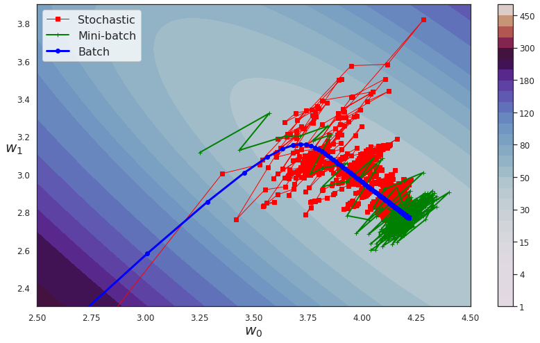
- All optimizers end up around the actual minima.
- Batch GD ends in the minima, while the other two end up around minima. They can reach the minima with appropriate learning schedule.
Visualization based diagnosis is not possible for real-word problems with more features, learning curves are our best friends in general case.
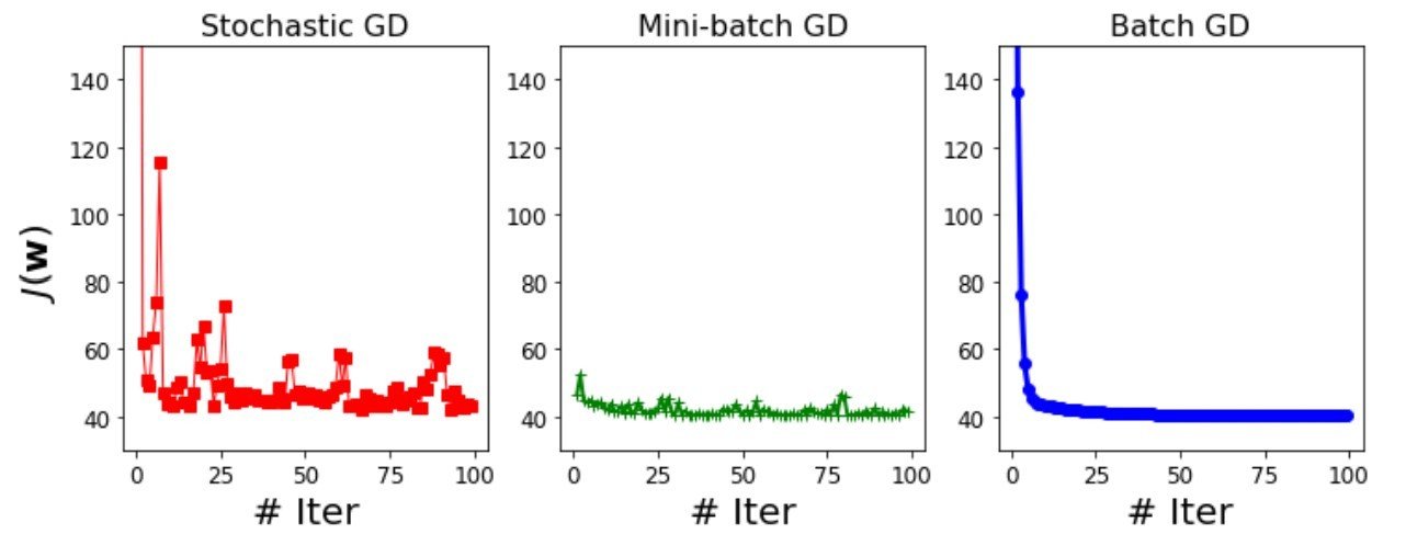
GD vs MBGD vs SGD: Learning curve comparison
GD vs MBGD vs SGD: Learning curve comparison
- Batch GD has the smoothest learning curve: the loss reduces continuously iterations after iterations.
GD vs MBGD vs SGD: Learning curve comparison
- The learning curves corresponding to mini-batch GD and SGD show ups and downs in loss.
- In some iteration, the loss reduces and then in the next one it goes up.
- Overall the losses are on downward trajectory.
GD vs MBGD vs SGD: Learning curve comparison
- As the batch size increases, the resulting learning curves become smoother for a given configuration of hyper-parameters like learning rate.
Evaluation
Evaluation
Uses root-mean-squared-error (RMSE) measure, which is derived from SSE.
Square-root is used to compare the error on the same unit and the same scale as that of the output label.
Division by \(n\), the size of the dataset, enables us to compare model performance on datasets of difference sizes on the same footing.
Linear regression: Recap
(1) Data
(2) Model
(3) Loss function
(4) Optimization procedure
(5) Evaluation
Sum of squared error (SSE)
Linear combination of features
Features and label that is real number.
(1) Normal eq. (2) GD/MBGD/SGD
Root mean squared error (RMSE)
Linear regression: Recap
(1) Data
(2) Model
(3) Loss function
(4) Optimization procedure
(5) Evaluation
\(J(\mathbf{w}) = \frac{1}{2} \left( \color{blue}{{\mathbf{X} \mathbf{w}}} \color{black}-\mathbf{y} \right)^T \left( \color{blue}{{\mathbf{X} \mathbf{w}}} \color{black}-\mathbf{y} \right) \)
\(h_\mathbf{w}: \mathbf{y} = \color{blue}{{\mathbf{X} \mathbf{w}}} \)
\( D = \left\{ (\mathbf{X}, \mathbf{y})\right\} = \left\{ (\mathbf{x}^{(i)}, y^{(i)})\right\}_{i=1}^{n} \)
(1) Normal eq. (2) GD/MBGD/SGD
Part II: Polynomial Regression
Why polynomial regression?
Many times the relationship between the input features and the output label is non-linear and simple linear models are not adequate to learn such mappings.
Polynomial regression: key idea
- The key idea is to create polynomial features by combining the existing input features.
- And then apply linear regression model on the polynomial feature representation.
Comparison: Linear and polynomial regression
\(\phi_k\)(features) is called polynomial transformation of \(k\)-th order.
Example: Polynomial transformation
- Let's assume that \((x_1, x_2)\) are two features.
- The second order polynomial transform\( \phi_2 (x_1, x_2) = (x_1, x_2, \color{blue}{x_1^2, x_2^2, x_1x_2}) \)
- The third order polynomial transform: \( \phi_3(x_1, x_2) = (x_1, x_2, x_1^2, x_2^2, x_1x_2, \color{blue}{x_1^3, x_2^3, x_1^2x_2, x_1x_2^2}) \)
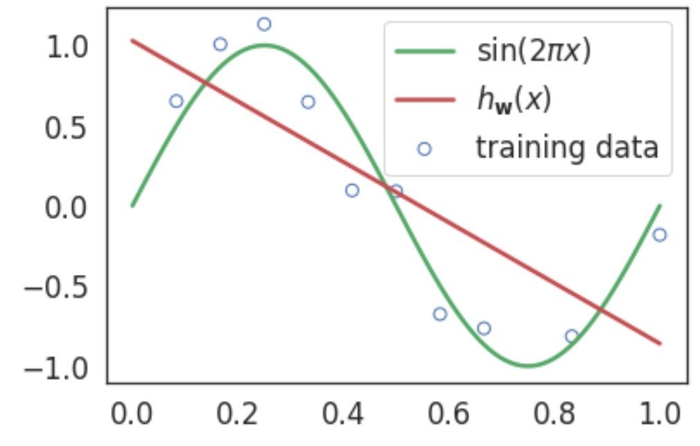
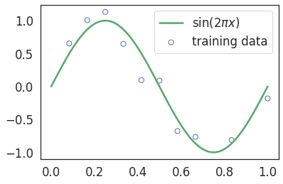
Polynomial regression: sample data

Linear regression without polynomial transformation.
Clearly, this is not a great fit and we need to search for a better model.
Why Polynomial Regression?
\(h_\mathbf{w}(x)=\color{red}w_0\color{black}+\color{red}w_1\color{black}x\)
In this case, we are able to visualize the model fitment since we are dealing with data in 1D feature space.
Fitness diagnostics
As the number of features grow, it won't be possible for us to visualize the fitment in this manner.
We rely on learning curve to determine quality of the fitment:
- Underfitting - both training and validation losses are high.
- Overfitting - training and validation losses decrease initially but then validation loss increases while training loss keeps decreasing.
Fitness diagnostics
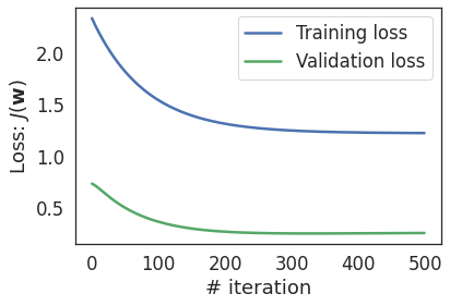
In this case, validation loss is less than the training loss (which is unusal), this is due to small amount of the validation data.
Learning curve of linear regression
Linear model underfits: it is not enough to model the relationship between features and labels as present in the training data.
How can we fix underfitting?
- By increasing the capacity of the model to learn non-linear relationship between the features and the label.
- One way to achieve it is through polynomial transformation that constructs new features from the existing features.
For training data with a single feature \(x_1\),
- First use \(k\)-th order polynomial transformation to create new features like \(x^2, x^3, \ldots, x^k \) and
- Use linear regression model to learn relationship between \(x_1\) and \(y\).
Polynomial regression in single feature
Note that the model is a non-linear function of \(x\), but is a linear function of weight vector \(\mathbf{w} = [w_0, w_1, \ldots, w_k]\).
Let's represent this transformation in form of a vector \(\mathbf{\phi}\) with \(k\) components.
Polynomial transformation
Each component denotes a specific transform to be applied to the input feature.
The polynomial regression model becomes:
Polynomial transformation: examples
- For a single feature \(x_1\), \(\phi_k = x_1^k\)
- Two features \((x_1, x_2)\), \(\phi_2(x_1, x_2) = \left[1, x_1, x_2, x_1^2, x_2^2, x_1x_2\right]\).
- Two features \((x_1, x_2)\), \(\phi_3(x_1, x_2) = \left[1, x_1, x_2, x_1^2, x_2^2, x_1x_2, x_1^3, x_2^3, x_1x_2^2, x_1^2x_2 \right]\)
- \(\phi_3\) contains features from \(\phi_2\).
Polynomial Transformation: Implementation
import itertools
import functools

def polynomial_transform(x, degree):
  '''Performs transformation of input x into deg d polynomial features.

  Arguments:
    x: Data of shape (n,)
    degree: degree of polynomial

  Returns:
    Polynomial transformation of x
  '''
  if x.ndim == 1:
    x = x[:, None]

  x_t = x.transpose()
  features = [np.ones(len(x))]
  for degree in range(1, degree + 1):
    for items in itertools.combinations_with_replacement(x_t, degree):
      features.append(functools.reduce(lambda x, y: x * y, items))
  return np.asarray(features).transpose()
Polynomial transformation: implementation
polynomial_transform(np.array([[1, 2], [3, 4]]), degree=3)An example:
array([[ 1.,  1.,  2.,  1.,  2.,  4.,  1.,  2.,  4.,  8.],
       [ 1.,  3.,  4.,  9., 12., 16., 27., 36., 48., 64.]])
Output:
Let's fit a polynomial model of different orders \( k =\{0, 1, 2, \ldots, 9\} \) on this data.
Fitting Polynomial Regression Models
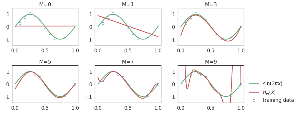
- Lower degree (0 and 1) polynomial model: Underfitting.
- Third order (degree=3) polynomial model: Reasonable fit.
- Higher degree \(\ge 7\) polynomial model: Overfitting.
Fitting Polynomial Regression Models
Model diagnostics: learning curves
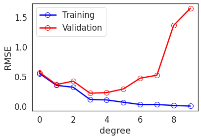
(1) Train polynomial model of degrees: \(\{0, 1, \ldots, k\}\)
(2) Calculate training and validation RMSE.
(3) Plot degree vs. RMSE plot.
Model diagnostics: learning curves
- The training and validation errors are close until certain degree.
- After a point, the training error continues to reduce, while the validation error keeps increasing.
- RMSE increases sharply for degrees \(\ge 7\). This is a signature of overfitting.
Issues with polynomial regression
- Higher order polynomial models are very flexible, or in other words, they have higher capacity compared to lower order models.
- Hence they are prone to overfitting compared to the lower degree polynomials.
- Perfect fit to training data, but poor prediction accuracy on validation data.
Demonstration of overfitting: deg = 9
Observe that higher degree polynomial features have higher weights than others.
\(h_\mathbf{w}(\mathbf{x})= \sum\limits_{j=0}^{j=9}w_jx^j\)
\(h_\mathbf{w}(\mathbf{x})= \sum\limits_{j=0}^{j=7}w_jx^j\)
Observe that higher degree polynomial features have higher weights than others.
Demonstration of overfitting: deg = 7
How to address overfitting?
- Using larger training sets.
- Controlling model complexity through regularization, which allows us to fit complex model on relatively smaller dataset without overfitting.
Fixing overfitting with more data
Train a polynomial model of degree 9 with two datasets - (i) with 15 points and (ii) with 100 points.

Smoother fitness
Overfitting is caused by larger weights assigned to the higher order polynomial terms.
Fixing overfitting through regularization
At a high level, let's modifies loss function by adding a penalty term as follows:
Regularization: Add a penalty term in the loss function for such large weights to control this behaviour.
Regularization modifies the loss function, which leads to the change in derivative of the loss function and hence a change in the weight update rule in gradient descent procedure.
Two components of regularization
- Penalty is a function of weight vector
- Regularization rate \(\lambda\) controls amount of penalty to be added to the loss function.
- L2 regularization (Ridge regression)
Regularization types
- L1 regularization (Lasso regression)
- Combination of L1 and L2: Elastic net regularization
Ridge Regression
Ridge regression uses second norm of the weight vector as a penalty term:
\(J(\mathbf{w}) = \frac{1}{2} \sum\limits_{i=1}^{n} (\mathbf{w}^T \mathbf{x}^{(i)} - y^{(i)})^2 + \frac{\lambda}{2} \sum_{i=1}^{m} w_i^2 \)
This can be written in a vectorized form as follows
Gradient calculation in ridge regression
These steps are same as gradient calculation in linear regression except for the penalty term.
Gradient calculation in ridge regression
Normal Equation
Let's set \(\dfrac{\partial J(\mathbf{w})}{\partial \mathbf{w}}\) to 0 and solving for \(\mathbf{w}\):
- [No regularization] When \(\lambda \rightarrow 0\), \(\mathbf{w} = \left( \mathbf{X}^T \mathbf{X} \right)^{-1} \mathbf{X}^T \mathbf{y}\) (Same as the linear regression solution)
- [Infinite regularization] When \(\lambda \rightarrow \infty \), \(\mathbf{w} = 0\)
Gradient Descent Update Rule
Effect of regularization \(\lambda\)
Effect of regularization \(\lambda\)
- As value of \(\lambda\) increases, the model loses its capacity and eventually for very large values of \(\lambda\), the model underfits the data.
Choosing \(\lambda\)
- Construct a set of values of \(\lambda\) that we want to experiment with.
- For each candidate value of \(\lambda\):
- Train the model and calculate cross validation error on validation set.
- Choose the the value of \(\lambda\) which results in the least cross validation error.
- With the chosen value of \(\lambda\), train the model on entire training set.
- Report the model performance on the test set.
\(\lambda\) vs Cross validation error
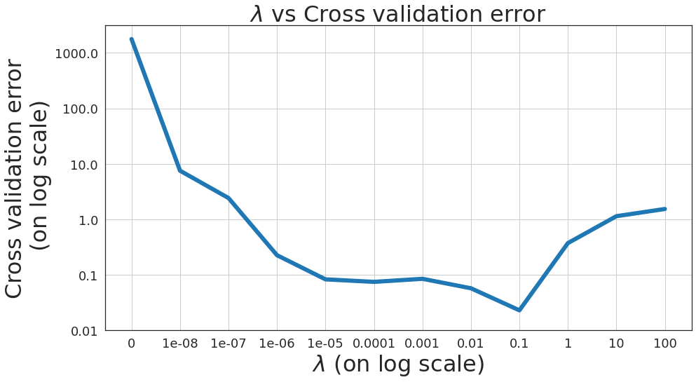
\(\lambda\) vs Cross validation error
Typically above chart looks like a bowl shape, however, due to small number of features and samples, the chart takes shape like above.
\(\lambda\) vs Cross validation error
The most appropriate value of \(\lambda\) results in lowest cross validation error.
\(\lambda\) vs Cross validation error
Most appropriate value of \(\lambda\) from above figure is 0.1.
Lasso Regression
We need specialized optimization algorithms to estimate weight vector in lasso regression, which are beyond scope of this course.
We will use sklearn implementation of Lasso in ML practice course.