Developing Deep Learning models
using PyTorch
(For Beginners)
Arun Prakash A
DEEP LEARNING
DEEP Neural Networks
Deeply Stacked Matrix Vector Products
ML
SVM
DT
PGM
KNN
DNN
Why do we need Deep Neural Networks?


Text
Natural Image

Video
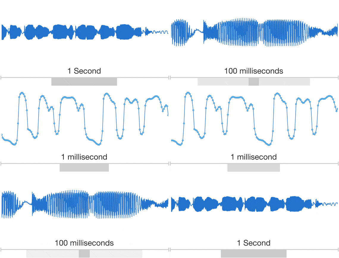
Speech
The data are Unstructured and DL models work really well with unstructured data (poorly for structured data)
One learning approach (Gradient based) for all these data types
Multi-Model: Paves the way to build a single model that learns from a two (or more) different modalities (Example: Image Captioning)
Model's performance scales up with increase in data size
Data type : Image
Dataset: CIFAR-10 (Natural images)
A single thread
Models: A single neuron, FCNN, CNN
Data Collection
Transformations
Training
model
Testing model



It is alright if some words are Alien to you
You may check my GitHub repo out if you want to go deeper into PyTorch.
Be One With Data
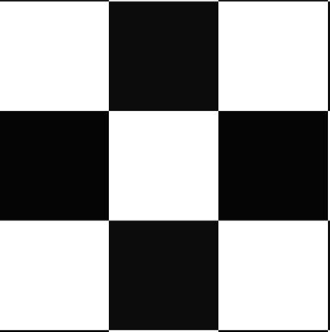
What we see
What A machine sees
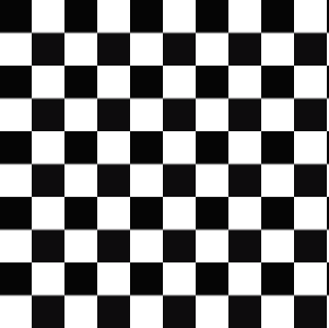

Matrix (Tensor) of dim \( m \times n \)
Image of size \(height \times width\)


Matrix (Tensor) of dim \( m \times n \)
Image of size \(height \times width\)


Matrix (Tensor) of dim \( m \times n \)
Image of size \(height \times width\)
R

G
B
R

G
B
Representing Text Data
" The course contents are well organized"
Tokenize
[The, course,contents,are,well,organized]
Numericalize
[{The:2, course:4,contents:1,are:3,well:5,organized:6}]Embedding
Requirements for DL Framework:
Ability to create \(n\) dimensional array or also called tensors
Scalar
(0 dim Tensor)
Vector
(1 dim Tensor)
Matrix
(2 dim Tensor)
Stacked Matrix
(3 dim Tensor)
Provide efficient ways to manipulate them (Accessing elements, mathematical operations, ..)
Most commonly used operations:
flatten()
reshape(1,9)
transpose(,0,1)
cat(,dim=1)
Most commonly used operations:
sum()
sum(,dim=0)
sum(,dim=1)
Scalar (dim=0)
Vector (dim=1)
Vector (dim=1)
Reduction Operations:
Mean, accessing elements
Most commonly used operations:
sigmoid()
softmax(,dim=0)


softmax(,dim=1)

across rows
across columns

Core: tensors
JIT
nn
Optim
multiprocessing
quantization
sparse
ONNX
Distributed
fast.ai
Detectron 2
Horovod
Flair
AllenNLP
torch.vision
BoTorch
GloW
Lightening
Skorch

Creating Tensors in PyTorch: Switch to colab
Why Image Recognition is a complex Task?

How many patterns are possible with an image of size \(3 \times 3\)?
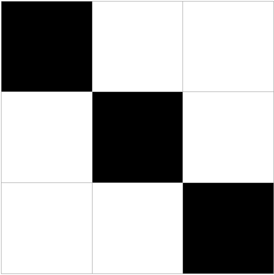


Of course, not all of them are relevant for a particular problem in most of the situation.
Recognize whether an image contains a single vertical line or not
The output is True for a very small subset of images and False for the rest
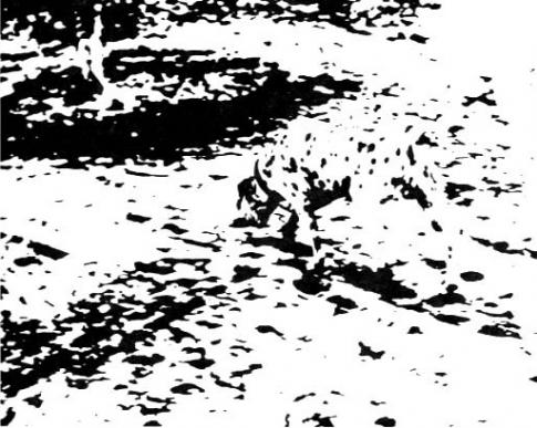
What do you perceive?
How many patterns are possible with an image of size \(5 \times 5\)?
How many patterns are possible with a colour image of size \(5 \times 5\)?
This is a challenge for Generative modelling
Our focus is on discriminative modelling
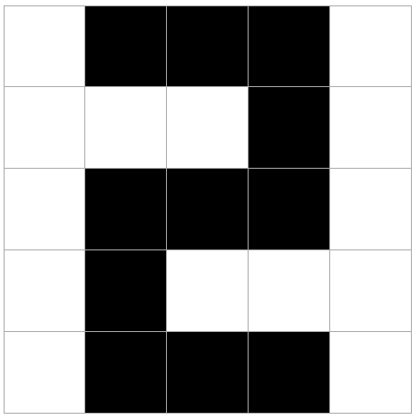
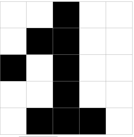
Two configurations out of million possibilities
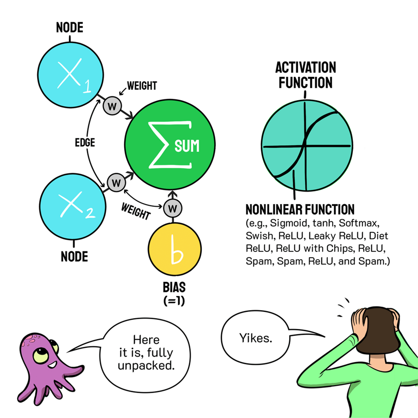
Neuron
The Parameter \(\mathbf{W}\) is randomly initialized
Compute the gradient of loss w.r.t \(\mathbf{w}\) , \(\nabla \mathbf{w}\)
Update rule:
The non-linear function \(f\) in neurons is called activation function
Check the performance with a set of criteria. Iteratively update the parameters for improving the performance
Wait, the image is not 1D then how do we feed it to a neuron as an input?

Note: Input elements are real-valued in general.
List of Activation functions
Few more design choices
- Loss functions
- Optimizers : SGD, Adaptive
- Hyper-parameters: Learning rate (schedulers), momentum, ..
Why do we need different Activation functions?
Just to ensure that the gradients flow across entire network
Feed Forward Neural Networks
(Multi-Layer (network of) Perceptron)
The input to the network is an \(n\)-dimensional vector
The network contains \(\text L-1\) hidden layers (2, in this case) having \(\text n\) neurons each
Finally, there is one output layer containing \(\text k\) neurons (say, corresponding to \(\text k\) classes)
\(a_2\)
\(a_3\)
Each neuron in the hidden layer and output layer can be split into two parts : pre-activation and activation (\(a_i\) and \(h_i\) are vectors)
\(x_1\)
\(x_2\)
\(x_n\)


pre-activation
(\(a_i\) and \(h_i\) are vectors)
The input layer can be called the \(0\)-th layer and the output layer can be called the (\(L\))-th layer
\(W_i \in \R^{n \times n}\) and \(b_i \in \R^n\) are the weight and bias between layers \(i-1\) and \(i (0 < i < L\))
\(W_L \in \R^{k \times n}\) and \(b_L \in \R^k\) are the weight and bias between the last hidden layer and the output layer (\(L = 3\)) in this case)
\(a_1\)
\(h_L=\hat {y} = \hat{f}(x)\)
\(h_2\)
\(h_1\)
\(W_1\)
\(W_1\)
\(b_1\)
\(W_2\)
\(b_2\)
\(W_3\)
\(b_3\)
and activation \(a_i\) and \(h_i\) are vectors)
The pre-activation at layer \(i\) is given by
\(a_i(x) = b_i +W_ih_{i-1}(x)\)
The activation at layer \(i\) is given by
\(h_i(x) = g(a_i(x))\)
where \(g\) is called the activation function (for example, logistic, tanh, linear, etc.)
The activation at the output layer is given by
\(f(x) = h_L(x)=O(a_L(x))\)
where \(O\) is the output activation function (for example, softmax, linear, etc.)
To simplify notation we will refer to \(a_i(x)\) as \(a_i\) and \(h_i(x)\) as \(h_i\)
\(a_2\)
\(a_3\)
\(x_1\)
\(x_2\)
\(x_n\)


\(a_1\)
\(h_L=\hat {y} = \hat{f}(x)\)
\(h_2\)
\(h_1\)
\(W_1\)
\(W_1\)
\(b_1\)
\(W_2\)
\(b_2\)
\(W_3\)
\(b_3\)
The pre-activation at layer \(i\) is given by
\(a_i = b_i +W_ih_{i-1}\)
The activation at layer \(i\) is given by
\(h_i = g(a_i)\)
where \(g\) is called the activation function (for example, logistic, tanh, linear, etc.)
The activation at the output layer is given by
\(f(x) = h_L=O(a_L)\)
where \(O\) is the output activation function (for example, softmax, linear, etc.)
\(a_2\)
\(a_3\)
\(x_1\)
\(x_2\)
\(x_n\)


\(a_1\)
\(h_L=\hat {y} = \hat{f}(x)\)
\(h_2\)
\(h_1\)
\(W_1\)
\(W_1\)
\(b_1\)
\(W_2\)
\(b_2\)
\(W_3\)
\(b_3\)
Data: \(\lbrace x_i,y_i \rbrace_{i=1}^N\)
\(\hat y_i = \hat{f}(x_i) = O(W_3 g(W_2 g(W_1 x + b_1) + b_2) + b_3)\)
Model:
\(\theta = W_1, ..., W_L, b_1, b_2, ..., b_L (L = 3)\)
Algorithm: Gradient Descent with Back-propagation
Objective/Loss/Error function: Say,
\(min \cfrac {1}{N} \displaystyle \sum_{i=1}^N \sum_{j=1}^k (\hat y_{ij} - y_{ij})^2\)
\(\text {In general,}\) \(min \mathscr{L}(\theta)\)
Parameters:
where \(\mathscr{L}(\theta)\) is some function of the parameters
\(a_2\)
\(a_3\)
\(x_1\)
\(x_2\)
\(x_n\)


\(a_1\)
\(h_L=\hat {y} = \hat{f}(x)\)
\(h_2\)
\(h_1\)
\(W_1\)
\(W_1\)
\(b_1\)
\(W_2\)
\(b_2\)
\(W_3\)
\(b_3\)
\(x_1\)
\(x_2\)
\(x_3\)
\(h_2\)
\(a_3\)
\(b_2\) = [0.01,0.02,0.03]
\(b_3\) = [0.01,0.02]
\(W_2\)
\(W_3\)
\(W_1=\)
\(a_2\)
\(h_1\)
\(a_1\)
1.5
2.5
3
\(W_2=\)
\(W_3=\)
0.36
0.37
0.38
0.589
0.591
0.593
0.054
0.064
0.074
0.513
0.516
0.518
1.558
1.568
0.497
0.502
\(\hat y = h_3 \)
\(\mathscr {L}(\theta) = -\frac{1}{N} \sum_{i=1}^N (y_ilog(\hat y_i)+(1-y_i)log(1- \hat y_i))\) = 0.6981
\(W_1\)
"Forward Pass"
\(x=[1.5, 2.5, 3]\)
\(b_1\) = [0.01,0.02,0.03]
\([h_1]=sigmoid(a_1)\)
\([h_2]=sigmoid(a_2)\)
\([h_3]=softmax(a_3)\)
\([a_1]=[1.5,2.5,3]*\)
\(+ [0.01,0.02,0.03]\)
\([a_2]=[0.589,0.591,0.593]*\)
\(+ [0.01,0.02,0.03]\)
\([a_3]=[0.513,0.516,0.518]*\)
\(+ [0.01,0.02]\)
\(y=[1, 0]\)
"Binary Cross Entropy Loss"


The weights are shared!

The weights are shared!

The weights are shared!

The weights are shared!

Convolution
Image
filter/kernel
Activation Map
A single neuron produce one activation map
The weights are shared!
Max Pooling
Recuurent Neural Networks
Sequence
"Text is something different from images"
Tokenizer
[Text,
is, something, different, from,
images]
Numericalize
Text is an ordered sequence
Embedding
Matrix
"Text:10"
Embedding
"Is:2"
Embedding
The weights are shared !
"Images:5"
Embedding
Replace a single by a layer of neurons!
The weights are shared !

Text is an ordered sequence
We want the model to capture the dependency!

DL-BootCamp-Sep2023
By Arun Prakash
DL-BootCamp-Sep2023
- 840


