Kolmogorov Arnold Network

Be a Game Changer?
Arun Prakash

The Problem
Given a set of \(N\) observations
(x_i,y_i)_{i=1}^N
0
6

coming from a true (solid blue) but unknown function
The Problem
Given a set of \(N\) observations
(x_i,y_i)_{i=1}^N
0
6
coming from a true (solid blue) but unknown function
Approximate the function from the observations
Approaches
Linear models (using the basis of standard Polynomials)
Neural Networks (MLP)
\vdots
Support Vector Machines (SVM)
taking a linear combination of the bases of (a standard) Polynomial function \((1,x,x^2,\cdots,x^n)\)
Approximate the function from the observations
f(x)=w_0+w_1x+w_2x^2+\cdots+w_nx^n
f(x)=\sum \limits_{p=1}^nw_p \color{blue}\phi_p(x)
Given a set of \(N\) observations
\{(x_i,y_i)\}_{i=1}^N
where
\color{red}\phi_p(x)=x^p
Polynomials
0
6

Basis : Global (fixed)
coming from a true (solid blue) but unknown function
\color{blue}\phi_p(x)=exp(-c(x-\mu_p)^2)
Look for bases that are local or adaptive to the training data
and B-splines
Bases are global functions of input variable (a small change around the region of a data point changes the approximated function globally )


Suffers a lot from Curse of Dimensionality (COD)
Neural Networks
Sigmoidal

For example,
Image source: PRML, Bishop
Neural Networks ( Universal Approximation Theorem UAT)
f(x)=\sum \limits_{p=1}^nw_p \color{blue}\phi_p(x)
Here, we let the neural network to learn the complex feature transformation \(\phi(x)\) via adaptive basis functions

With \(N=50\) data points
Learned Bases (Activation functions) of a neuron in a hidden layer with 3 units
Neuron-1
Neuron-2
Neuron-3
Image source: PRML, Bishop
Neural Networks ( Universal Approximation Theorem UAT)
f(x)=\sum \limits_{p=1}^nw_p \color{blue}\phi_p(x)
Here, we let the neural network to learn the complex feature transformation \(\phi(x)\) via adaptive basis functions
With \(N=50\) data points
Learned Bases (Activation functions) of a neuron in a hidden layer with 3 units
Neuron-2
Neuron-3
Neuron-1
Ultimately, it is all about combining the activation functions to approximates the true function at observed points

Image source: PRML, Bishop
MLP-Neural Networks ( Universal Approximation Theorem UAT)
UAT: With One (hidden) layer NN
\hat{f}(\mathbf{x}) \approx \sum \limits_{i=1}^{N(\epsilon)}\alpha_i\sigma(W_i^T\mathbf{x}+b)
We can approximate any continuous function to desired precision \(\epsilon\)
z=w^Tx
For a single neuron

z
Here the activation (basis) function \(\sigma\) is Fixed
The adaptability to the data is due to the learnable parameters \(w\)
f(x)=\sum \limits_{p=1}^nw_p \color{blue}\phi_p(x)
Here, we let the neural network to learn the complex feature transformation \(\phi(x)\) via adaptive basis functions
Image source: DL Lectures by Mitesh Khapra
So, what are the problems with MLPs?
Interpretability is difficult with the vast number of learnable weights \(w\)
Continual learning without re-training is difficult
Catastrophic forgetting due to fixed and non-local activation functions
Sparsification and pruning are difficult due to large number of parameters
KAN overcomes (at least in toy settings) all of these
Adaptive Basis functions are all we need
Consider a multivariate function \(f(\mathbf{x})\) with \(\mathbf{x} \in \mathbb{R}^n\), \((x_1,x_2,\cdots,x_n)\)
x_1 \in \mathbb{R}


{z}_1 \in \mathbb{R}
z_2 \in \mathbb{R}
Bold cliam: Any continuous smooth multivariate function \(f(\mathbf{x})\) can be represented using \(n\) univariate functions \(\phi_p(x_p), p=1,2,\cdots,n\)
\phi_2(x_2)
\phi_1(x_1)
x_2 \in \mathbb{R}
Is \(\phi_p(x_p)\) fixed or learnable? Learnable
How do we combine the output from the \(n\) univariate functions to get \(f(\mathbf{x})\)?
\cdots

\phi_n(x_n)
z_n \in \mathbb{R}
x_n \in \mathbb{R}
\cdots
\cdots
f(x_1,x_2,\cdots,x_n)=
\sum \limits_{q=1}^{2n+1}\Phi_q
\sum \limits_{p=1}^{n}\color{blue}\phi_{p}(x_p)
Kolmogorov Representation Theorem
x_1 \in \mathbb{R}
\cdots
{z}_1 \in \mathbb{R}
z_2 \in \mathbb{R}
\phi_n(x_n)
\phi_2(x_2)
\phi_1(x_1)
z_n \in \mathbb{R}
x_2 \in \mathbb{R}
x_n \in \mathbb{R}
\cdots
\cdots
Sum the outputs from all univariate functions
In reality, we need \((n(2n+1))\) \(\phi\)s and (\(2n+1 \)) \(\Phi_q\)s, totaly \(2n^2+3n+1\) learnable univarate functions (not just \(n\) as claimed in the previous slide)
\bigg(\sum \limits_{p=1}^{n}\color{blue}\phi_{qp}(x_p) \color{black}\bigg)
\mathbb{R}
[0,1]
\mathbb{R}
\mathbb{R}
Well, How do we make a learnable 1D function?
Hey, B-splines
B-Spline Functions
\phi(x)=\sum \limits_{i=0}^nB_{i}(x)c_i
A function in the basis \(B\)
\(c_i \in \mathbb{R}\): spline coefficeints (control points)
\(B_i(x)\): The basis function of order \(k\) (degree \(d=k-1\))
\(t=(t_{-k},\cdots,t_{G+k})\): Uniformly spaced knots (think of this as a uniformly spaced grid of points defined by \(G\))
\(c_i \)'s are learnable parameters (initialized randomly based on the problem)

G=5
[t_{-k+i},t_{i+1}]
Basis support:
G+k-1
d=?

k=3
G=5
x \in [-1,1]
h= \frac{x[1]-x[0]}{G}=\frac{2}{5}=0.4
t=[-k:G+k]=[-3,-2,-1,\cdots,8]
h=0.4
(k+1)*h=1.6
Spline width = \((k+1)*h=1.6\)
Increasing the value of \(G\) decreases \(h\) and hence the width of the splines ( sort of controlling the resolution)
?
k=3
G=5
x \in [-1,1]
h= \frac{x[1]-x[0]}{G}=\frac{2}{5}=0.4
t=[-k:G+k]=[-3,-2,-1,\cdots,8]
grid=t*h+ (-1)
offset by starting value of x
[-2.2,-1.8,-1.4,-1,-0.6, \cdots 1, 1.4,1.8,2.2]
[-2.2,-1.8,-1.4,-1,\cdots
The grid extends on both sides with the basis function
h=0.4
Building KAN with \(n=2\) inputs
x_{01}
x_{02}
w_{ijk}
Each* learnable weight \(w_{ijk}\) in MLP is replaced by an learnable activation \(\phi_{ijk}\) as shown in the figure right

Each node sums the incoming values
*Not replacing bias (as it is not function of input)
\sigma
\sigma
\sigma
\sigma
\sigma
\sum \limits_{q=1}^{5}\Phi_q
\bigg(\sum \limits_{p=1}^{2}\color{blue}\phi_{qp}(x_p) \color{black}\bigg)
\Phi_5\bigg(\phi_{51}(x_1)+\phi_{52}(x_2)\bigg)
A term in the outer summation
\sigma
KAN-Layer-1
\(n \to 2n+1\)
KAN-Layer-2
\(2n+1 \to 1\)
n
2n+1
1
x_{01}
x_{02}
w_{ijk}
Number of parameters:
*Not replacing bias (as it is not function of input)
\sigma
\sigma
\sigma
\sigma
\sigma
\sigma
15 (ignoring bias)
k=3,G=5
For each function
Therefore, 15*(5+3)=120
Number of coefficients: \(c=G+k\)
What more parameters than MLP?
Building KAN with \(n=2\) inputs
\Phi_1=\begin{bmatrix} \phi_{11}() & \phi_{12}() \\
\phi_{21}() & \phi_{22}() \\
\vdots \\
\phi_{51}() & \phi_{52}()\end{bmatrix}
\begin{bmatrix} x_1 \\ x_2 \end{bmatrix}
x_{01}
x_{02}
w_{ijk}
Number of parameters:
*Not replacing bias (as it is not function of input)
\sigma
\sigma
\sigma
\sigma
\sigma
\sigma
15 (ignoring bias)
15*(8)=120
What more parameters than MLP?
However, often, it requires less number of KAN layers than MLP Layers
Building KAN with \(n=2\) inputs
Generalized KAN
\(2n^2+3n+1\) learnable functions are sufficient if we are able to find the correct \(\phi(x)\) that represents \(\mathbf{f(x)}\).
But, \(\mathbf{f(x)}\) is not known. Moreover, we choose smooth B-splines (among other non-smooth alternatives like fractals) to learn \(\phi(x)\)
Therefore, to get a better approximation, one can build KAN with arbitrary width and depth ( replacing weights by learnable activations)
The author mentions "To the best of our knowledge, there is not yet a “generalized” version of the theorem that corresponds to deeper KANs"
However, they do derive the approximation theory for KAT assuming \(k-th\) order B-splines for all \(\Phi\)s.
Deep MLP vs KAN

MLP(\mathbf{x})= (W_3 \circ \sigma_2 \circ W_2 \circ \sigma_1 \circ W_1)\mathbf{x}

KAN(\mathbf{x})= (\Phi_3 \circ \Phi_2 \circ \Phi_1)\mathbf{x}
Optimization: Backpropagation
Optimization : Backpropagation, (LBFGS for small networks)
\phi(x)=w(b(x)+spline(x))
Training tricks: Residual connection
Training tricks:
b(x)=\frac{x}{1+e^{-x}}
(silu),\(w\) learnable
Initialization: Typically, Xavier
Initialization: Xavier for \(w\), \(N(0,0.1)\) for \(c_is\)
KAN and Scaling Law
Loss: \(L \propto N^{-\alpha}\)
The higher the value of \(\alpha\) for the model parameters \(N\), the lower the loss. We can get quick improvement by scaling the model parameters
How do we predict \(\alpha\)?
Different theories: relating to intricate dimensionality of data \(d\) (need to ponder over this), as a function of the class activations.
Function class: Order \(k\) of piecewise polynomial like ReLU ( \(k=1\)), (Maxout?)
\alpha=\frac{k+1}{d}
For KAN: B-Splines with order \(k=3\) gives \(\alpha = 4\) (independent of \(d\))
Increasing the number of parameters in KAN reduces the loss quickly than MLP (albeit with more computations)
Fine Graining by Grid Extension

(G+k-1)
t_{-k}
t_{G+k}
Uniform Grid intervals (knots)
Splines can adjust its resolution (like wavelets)
Coarse Resolution
Fine Resolution

One can increase the grid size (therefore number of parameters) on the fly during training (without re-training from scratch)
As per scaling law for KAN, the loss \(L \propto N^{-4}\) should reduces quickly
Unique to KAN
by varying the Grid size \(G\)
Validated in a toy setting
Fine Graining by Grid Extension
(G+k-1)
t_{-k}
t_{G+k}
Uniform Grid intervals (knots)
Splines can adjust its resolution (like wavelets)
by varying the Grid size \(G\)
Target
An estimator
Use least squares to solve this
Fine Graining by Grid Extension
(G+k-1)
t_{-k}
t_{G+k}
Uniform Grid intervals (knots)
Splines can adjust its resolution (like wavelets) with the Grid size \(G\)
One can increase the grid size (therefore number of parameters) on the fly during training (without re-training from scratch)

f(x,y)=exp(sin(\pi x)+y^2)
Unique to KAN
As per scaling law for KAN, the loss \(L \propto N^{-4}\) should reduces quickly
Fine Graining by Grid Extension
(G+k-1)
t_{-k}
t_{G+k}
Uniform Grid intervals (knots)
Splines can adjust its resolution (like wavelets) with the Grid size \(G\)
One can increase the grid size (therefore number of parameters) on the fly during training (without re-training from scratch)
As per scaling law for KAN, this should reduces the loss quickly
Unique to KAN
KAN trains the network continually without catastrophic forgetting (Caution: not trained and tested on NLP tasks)
Continual Learning
WE can play around with different basis


External Vs Internal Degree of Freedom (DoF)
Refer to page 10 and 11 of the paper for details
External DoF: Composition (like MLP) of layers
Internal DoF: Grid size (Unique to KAN)
Sparsification and Pruning
Given the samples from known function structure, the network learns the structure via sparsification and pruning.

Since we do not have linear weights. The \(L_1\) norm is computed for each KAN layer \(\Phi()\)
Here the target function contains three (activation) functions (exp,sin,parabola)
However, the KAN layers have 15 activations
Can it only learn those three out of 15 activation functions?
Sparsification and Pruning
Given the samples from known function structure, the network learns the structure via sparsification and pruning.
Since we do not have linear weights. The \(L_1\) norm is computed on \(\Phi()\) matrices.
(x_i)_{i=1}^{N_p}
|\phi|_1= \frac{1}{N_p}\sum_i |\phi(x_i)|
Norm for an activation is given by
Norm for the layer \(\Phi\)
\Phi_1=\sum \limits_{i}^{n_{in}} \sum \limits_{j}^{n_{out}} |\phi_{i,j}|_1
Sparsification and Pruning
Given the samples from known function structure, the network learns the structure via sparsification and pruning.
Since we do not have linear weights. The \(L_1\) norm is computed on \(\Phi()\) matrices.
Sparsification and Pruning
Given the samples from known function structure, the network learns the structure via sparsification and pruning.
Since we do not have linear weights. The \(L_1\) norm is computed on \(\Phi()\) matrices.
Interpretability
Suppose the function structure is unkown
After training, we end up with this simple structure
Then we could infer that the target function contains only three univariate functions
Continual learning and Catastrophic forgetting
Humans are good at multi-tasking without fogetting any of the tasks when learning a new task
human brains have functionally distinct modules placed locally in space
Most artificial neural networks, including MLPs, do not have this notion of locality, which is probably the reason for catastrophic forgetting.
KANs have local plasticity and can avoid catastrophic forgetting by leveraging the locality of splines (a sample will only affect a few nearby spline coefficients, leaving far-away coefficients intact)
Let's validate this via a simple 1D regression task composed of 5 Gaussian peaks

Continual learning and Catastrophic forgetting
Data around each peak is presented sequentially (instead of all at once)
Continual learning and Catastrophic forgetting
Data around each peak is presented sequentially (instead of all at once)
Continual learning and Catastrophic forgetting
Data around each peak is presented sequentially (instead of all at once)
Slow to train.KANs are usually 10x slower than MLPs, given the same number of parameters
Limitations
Findings are validated using Toy experimental settings that are closely related to maths and physics.
They left it to engineers to optimize (efficient implementations have already started emerging)

When to use KAN?

Playground to get started with
What is your take on KAN?

What are Splines?
Splines with control points
c_0
c_1
(1-t)c_0+t c_1
t \in [0,1]
t=0
t=0.5
t=1
A line segment is parameterized by \(t\) (convex combination of the control points (\(c_0,c_1\)))
q(t|c_0,c_1,t_0,t_1)=\frac{t_1-t}{t_1-t_0}c_0+\frac{t-t_0}{t_1-t_0}c_1
t \in [t_0,t_1]
and
t_0< t_1]
A line segment
q_{0,1}(t)=q(t|c_0,c_1,t_0,t_1)=\frac{t_1-t}{t_1-t_0}c_0+\frac{t-t_0}{t_1-t_0}c_1
A quadradic curve
Control points : \(c_0,c_1,c_2\)
t : \(t_0,t_1,t_2\) , \(t_0<t_1<t_2\)
c_0
c_1
c_2
q_{1,2}(t)=q(t|c_1,c_2,t_1,t_2)=\frac{t_1-t}{t_1-t_0}c_0+\frac{t-t_0}{t_1-t_0}c_1
Construct two line segments
Then the curve is given by
q_{0,2}(t)=q(t|c_0,c_1,c_2,t_0,t_1,t_2)=\frac{t_2-t}{t_2-t_0} \color{blue} q_{0,1}(t) \color{black}+\frac{t-t_0}{t_2-t_0}\color{blue}q_{1,2}(t)
q_{0,1}(t)
q_{1,2}(t)
Splines with control points
q_{0,1}(t)=q(t|c_0,c_1,t_0,t_1)=\frac{t_1-t}{t_1-t_0}c_0+\frac{t-t_0}{t_1-t_0}c_1
A quadradic curve
Control points : \(c_0,c_1,c_2\)
t : \(t_0,t_1,t_2\) , \(t_0<t_1<t_2\)
c_0
c_1
c_2
q_{1,2}(t)=q(t|c_1,c_2,t_1,t_2)=\frac{t_1-t}{t_1-t_0}c_0+\frac{t-t_0}{t_1-t_0}c_1
Construct two line segments
Then the curve is given by
q_{0,2}(t)=q(t|c_0,c_1,c_2,t_0,t_1,t_2)=\frac{t_2-t}{t_2-t_0} \color{blue} q_{0,1}(t) \color{black}+\frac{t-t_0}{t_2-t_0}\color{blue}q_{1,2}(t)

t=(0,1,2)
Splines with control points
q_{0,1}(t)=q(t|c_0,c_1,t_0,t_1)=\frac{t_1-t}{t_1-t_0}c_0+\frac{t-t_0}{t_1-t_0}c_1
A quadradic curve
Control points : \(c_0,c_1,c_2\)
t : \(t_0,t_1,t_2\) , \(t_0<t_1<t_2\)
c_0
c_1
c_2
q_{1,2}(t)=q(t|c_1,c_2,t_1,t_2)=\frac{t_1-t}{t_1-t_0}c_0+\frac{t-t_0}{t_1-t_0}c_1
Construct two line segments
Then the curve is given by
q_{0,2}(t)=q(t|c_0,c_1,c_2,t_0,t_1,t_2)=\frac{t_2-t}{t_2-t_0} \color{blue} q_{0,1}(t) \color{black}+\frac{t-t_0}{t_2-t_0}\color{blue}q_{1,2}(t)
t=(0,0.5,2)

unlike for line segment, choice of \(t\) (parameters) affects the shape of curve
Splines with control points
Polynomial Splines may not always be smooth

We need to be carefult about the choice of intervals to get a smooth curves
Solution?
Splines - Bezier Curves
Control points \(n=3\): \(c_i, i=0,1,2\)
t : \(t_0,t_1,t_2\)
The interval is restricted to [0,1] (convex combination)

p_{0,1}(t)=(1-t)c_0+tc_1
p_{1,2}(t)=(1-t)c_1+tc_2
FInal curve is the convex combination of above
p_{0,2}(t)=(1-t)p_{0,1}(t)+tp_{1,2}(t)
p_{0,2}(t)=(1-t)^2c_0+2t(1-t)c_1+t^2c_2
Substitute the expresssion for \(p_{0,1},p_{1,2}\)
c_0
c_1
c_2
p_{0,2}(t)=b_{02}(t)c_0+b_{12}(t)c_1+b_{22}(t)c_2
\text{degree},d=2
p_{0,2}(t)=\sum \limits_{i=0}^2b_{i,d}(t)c_i
It is smooth
p_{0,2}(t)=\sum \limits_{i=0}^2b_{i,d}(t)c_i
We can generalize this to degree \(d\) and \(n\) control points
P(t)=\sum \limits_{i=0}^nB_{i,d}(t)c_i
Where \(B_{i,d}(t)\) is a basis function for \(c_i\)
d \choose i
B_{i,d}(t)=
t^i(1-t)^{d-i}
For example, it is a Bernstein Polynomials for Bezier curves
Basis-Spline
p_{0,2}(t)=(1-t)^2c_0+2t(1-t)c_1+t^2c_2
p_{0,2}(t)=b_{02}(t)c_0+b_{12}(t)c_1+b_{22}(t)c_2
Quick Check for \(n=3, d=n-1\)
p_{0,2}(t)=\sum \limits_{i=0}^2b_{i,d}(t)c_i
We can generalize this to degree \(d\) and \(n+1\) control points
P(t)=\sum \limits_{i=0}^nB_{i,d}(t)c_i
In the case of B-Splines, it is a called Blending functions described by order \(k=d+1\) with a non-decreasing sequence of numbers called knots \(t_i: i=0,1,2,\cdots n+k\)
Let us try to understand this with illustrations (borrowed from Kenneth)
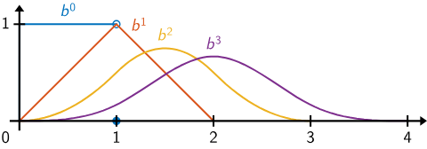
From curves to B-Spline Functions
Let us start with first order \(k=1\) constant \(d=0\) piecewise polynomial functions
B-Splines \(B_{i,0}(t)\), knots \(t_i\) are uniformly spaced in the interval [0,1].

\(B_{0,0}(t)\)

\(B_{1,0}(t)\)
The first degree (\(d=1\)) spline is obtained by combining the first order splines
The function for the \(i-th\) control point (or knot) is simply a shifted version of \(B_{0,d}(t)\) by \(i\) units
Image source: Lectures by Kenneth I Joy
B-Splines \(B_{i,1}(t)\), knots \(t_i\) are uniformly spaced in the interval [0,1].

Note the increase in support for the function as the order increases
The quadratic (third order) spline is obtained by combining the second order splines
\(B_{0,1}(t)\)
Image source: Lectures by Kenneth I Joy

B-Splines \(B_{i,2}(t)\), knots \(t_i\) are uniformly spaced in the interval [0,1].
\(B_{0,2}(t)\)
\(B_{1,2}(t)\)
Image source: Lectures by Kenneth I Joy

P(t)=\sum \limits_{i=0}^nB_{i,d}(t)c_i
Now treat \(c_i \in \mathbb{R}\) as a real number
Now, the curve \(P(t)\) is learnable via \(c_i\)
The number of control points \(c_i\) and the order \(k=d+1\) are independent.
B-Spline Functions
Now, \(c_i\) is called B-Spline coefficient
For rigours definition and proofs: here
References
Kolmogorov-Arnold-Networks (KAN)
By Arun Prakash
Kolmogorov-Arnold-Networks (KAN)
Intro to KAN


