Linear Regression - Kernel Regression
Arun Prakash A
Supervised: Samples \(X\) and Label \(y\)
Regression
Classification
Binary
Multiclass
Simple/Multiple
Multivariate
Multilabel
Dataset : \(\{X,y\}\)
\(n\) samples, \(d\) features
\(y\) target/label
A single training example is a pair \(\{x_i,y_i\}\)
features
samples
Supervised Learning: Regression
Dataset : \(\{X,y\}\)
Example: \(d=1\)

We can either treat the feature "price" or the feature " living area in square feet" as a target variable \(y\)
True or False?
\(n\) samples, \(d\) features
\(y\) target/label
A single training example is a pair \(\{x_i,y_i\}\)
Example: \(d=1\)

We can either treat the feature "price" or the feature " living area in square feet" as a target variable \(y\)
True or False?
Regression is always linear.
True or False?
Assume a Linear relation
Let's write it compactly!
Set the gradient to zero to find \(w^*\)
Use pseudo inverse if inverse doesn't exist ( because pseudo inverse matrix satisfies all the properties that an inverse matrix satisfy )
Hessian. If \(XX^T\) is PSD, the solution is unique
Info Byte
That is, the columns of \(X\) has to be linearly independent

is called the projection matrix


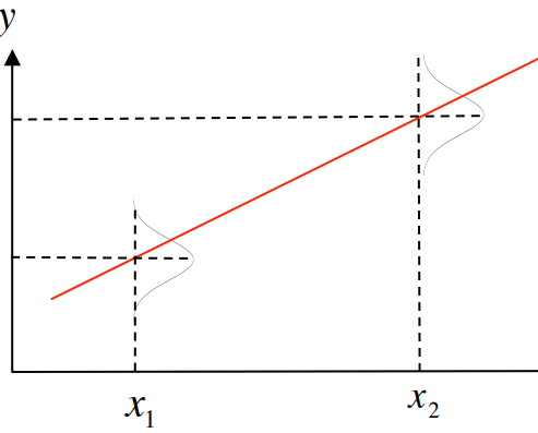
From Deterministic to Random
We are not sure whether the observed \(d\) features are sufficient to explain the observed \(y\) .
We might have missed some features (correlated or uncorrelated) that could potentially relate to \(y\)
We could model this as a random variable \(\epsilon\) (or noise), that could explain the deviation in the prediction.
\(\epsilon\) could follow any distribution, generally assumed to be normal if not specified otherwise
This gives a fixed value for \(y\) for given \(x\) .
However, we can see that prediction deviates from the actual values. (there could be more than one value for \(y\) for given \(x\))
Now, the prediction is the expectation of \(y,E[y|x]\) (the value of \(y\) on an average for the given \(x\))
This gives us
mean
Likelihood of \(y\) given \(x\)
Maximize log-likelihood
Maximizing the log-likelihood is equivalent to minimizing the sum square error.
Computational complexity
Complexity: \(O(d^3)\), requires all samples
Use an iterative algorithm: Gradient Descent
Initialize \(w\) randomly and compute the gradient
Update \(w\)
Repeat until the loss (or gradient) becomes zero.
Go with stochastic gradient descent if we do not have enough compute.
Non-Linear Regression (Kernel Regression)

Fit datapoints globally
Linear regression
Kernel Regression
w.k.t
Computing \(XX^T\) is costly for \(d>>n\)
Manipulating it further
during testing

w.k.t
Kernel maps the data points to infinite dimension, then it requires infinite number of parameters in the transformed domain. So, does it always overfit the training data points.?
No. It overfits when \(K\) has a full rank (therefore, inverse exists). In practice, it rarely occurs when we have number of samples equals to the number of features
Summary of Important concepts
Supervised: Samples \(X\) and Label \(y\)
Regression
Classification
Binary
Multiclass
Simple/Multiple
Multivariate
Multilabel
Data : \(\{X,y\}\)
features
samples
Linear Regression: Solving via Normal Equations
Model : Linear
Loss : Squared Error Loss
\(w=w^*\) that minimizes the loss

is called the projection matrix
From Deterministic to Random
We could model this as a random variable \(\epsilon\) (or noise), that could explain the deviation in the prediction.
mean
Likelihood of \(y\) given \(x\)
Maximize log-likelihood
Maximizing the log-likelihood is equivalent to minimizing the sum square error.
Computational complexity
Complexity: \(O(d^3)\), requires all samples
Use an iterative algorithm: Gradient Descent
Initialize \(w\) randomly and compute the gradient
Update \(w\)
Stop the iteration based on some criteria (such as number of iterations, loss_threshold..)
Go with stochastic gradient descent if we do not have enough compute.
Linear regression
Kernel Regression
w.k.t
Computing \(XX^T\) is costly for \(d>>n\)
Manipulating it further
during testing
Linear Regression - Kernel Regression - ProbabilisticView
By Arun Prakash
Linear Regression - Kernel Regression - ProbabilisticView
MLT - Week5 Session slides
- 666


