Module 4 : Prefer Pre-Norm to Post-Norm


AI4Bharat, Department of Computer Science and Engineering, IIT Madras
Mitesh M. Khapra
Motivation
Recall that vanilla transformer architecture uses a warmup learning rate strategy to make the training process stable during initial time steps

warmupSteps=4000
Moreover, the "no. of warmup steps" becomes another hyperparameter that needs to be carefully tuned
But, why did the training become unstable in the first place for transformer models?
Typically, in CNN and RNN networks, the learning rate starts with a high value and gradually decreases over iterations
Starting with a very small learning rate implies that the gradient values might be large, and small learning rate counters that to make the training stable
This slows down the optimization process due to very small initial rate for a few initial time steps
Well, the scale of gradients also depends on the scale of inputs. So normalization might play a role!
Post Normalization

Given a sequence of vectors \([x_1,\cdots,x_T]\), we denote
\text{MHA}(x_i,[x_1,\cdots,x_T])
multi-head attention applied on the sequence at \(i-\)th position from \(x_i\) to all other tokens
then we add a residual connection
r_i=x_i+\text{MHA}(x_i,[x_1,\cdots,x_T])
then the layer norm is computed as follows
LN(r_i)=\gamma \frac{r_i-\mu}{\sigma}+\beta
where \(\gamma\) and \(\beta\) are parameters
This is called post normalization
Post Normalization


The total computation steps (1,2,3,4,5) for \(l-th\) layer and \(i-th\) position with \(n\) heads are given in the table below
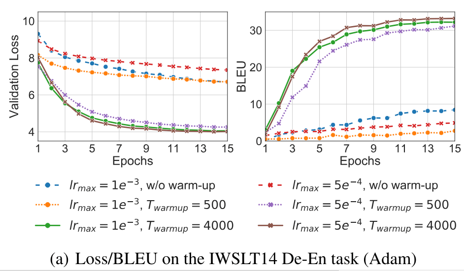
Let's see how the validation loss and BLEU score changes with and without warm-up for various initial learning rates

Without warm-up, the loss remained between 8-7 and the model was able to achieve a BLEU score of only 8.45
\(T_{warmup}=4000\) acheives better BLEU score than \(T_{warmup}=500\)

Without warm-up, the loss remained between 8-7 and the model was able to achieve a BLEU score of only 8.45
\(T_{warmup}=4000\) acheives better BLEU score than \(T_{warmup}=500\)
Now, let us try to understand how warm-up helps the training process and if there is a way to drop this strategy altogether
Note that we are going to analyze the behaviour of gradient values for a few initialization steps. So we can reasonably assume that the weights and inputs are all coming from Gausian distribution
(because the values are initialized randomly for both embeddings and parameters)
Pre- Normalization
Post-LN puts the LN block between the residual block (addition-addition) whereas pre-LN relocates it as shown in the figure

Post-LN
Pre-LN
It simply normalizes the input before passing it to the self-attention or FFN layers (it intuitively makes sense). Additionally, pre-LN is applied in the final layer right before the prediction
But, why does this small modification eliminate the need for a warm-up strategy and lead to better performance when \(L\) is large?
For that, we need to understand the behaviour of gradient values during the initial few steps
It outperforms post-LN especially when the number of layers \(L\) increases
This [paper] shows that the scale of the gradients of weights in the last \((L-th)\) FFN layer for the model using post-norm is given by
||\frac{\partial \mathcal{L}}{\partial W_2^{L}}||_F\leq O\bigg(d\sqrt{ln \ d}\bigg)
||\frac{\partial \mathcal{L}}{\partial W_2^{L}}||_F\leq O\bigg(d\sqrt{\frac{ln \ d}{L}}\bigg)
whereas, the scale of the gradients of weights in the last \((N-th)\) FFN layer for the model using pre-norm is given by
Let the shape of \(W_Q^l,W_K^l,W_V^l, W_O^l\) and the weights of FFN (\(W_1^l,W_2^l\)) be \(d_{model} \times d_{model}\) . That is, only a single head-attention is used in all layers (\(l=1,2,\cdots,L\))
This clearly shows that the scale of the gradients decreases as the number of layers increases and hence the usage of warm-up strategy may not be required.
Recall that the scale of gradient depends on the scale of inputs as well. It is shown that the scale of the inputs are bounded under certain reasonable assumptions
||\frac{\partial \mathcal{L}}{\partial W_2^{L}}||_F\leq O\bigg(d\sqrt{ln \ d}\bigg)
||\frac{\partial \mathcal{L}}{\partial W_2^{L}}||_F\leq O\bigg(d\sqrt{\frac{ln \ d}{L}}\bigg)
Post-LN
Pre-LN
Let the shape of \(W_Q^l,W_K^l,W_V^l, W_O^l\) and the weights of FFN (\(W_1^l,W_2^l\)) be \(d_{model} \times d_{model}\) . That is, only a single head-attention is used in all layers (\(l=1,2,\cdots,L\))

W_1^l
W_2^l
Without warm-up in post-LN, the expected gradient value of \(W_1,W_2\) grows with \(L\). This makes the training process unstable.
One can also fix this issue with a suitable optimization algorithm like Rectified ADAM(RADAM)
Performance

As we can see, in any case (RADAM vs ADAM, with or without warm-up), using pre-LN helps the model converge faster.
Notations
\(\mathcal{L_i}()\) be a loss value for one position
\(\mathcal{L}()\) be a total loss
\(LN(x)\) be a layer normalization of \(x\) with \(\beta=0, \gamma=1\)
\(\mathbf{J}_{LN(x)}=\frac{\partial LN(x)}{\partial x}\) be a Jacobian of \(LN(x)\)
Typically, we use Xavier Initialization
Given a matrix of size \(n_{in},n_{out}\), the xavier initialization sets the value of each element by sampling from Gausian distribution
N(0,\frac{2}{n_{in}+n_{out}})
The shape of \(W_Q,W_K,W_V, W_O\) and the weights of FFN \(W_1,W_2\) be \(d_{model} \times d_{model}\) . That is, only a single head-attention is used
Moreover, assume that \(W_Q,=W_K=\mathbf{0}\) . Therefore, the attention matrix \(A\) follows a uniform distribution. Thus the new representation is given by
z_i=\frac{1}{T}\sum x_iW_v
Reference
PostNorm-vs-PreNorm
By Arun Prakash
PostNorm-vs-PreNorm
- 1,541


