Lecture 2: Language Modelling, GPT, Decoding Strategies


AI4Bharat, Department of Computer Science and Engineering, IIT Madras
Introduction to Large Language Models
Mitesh M. Khapra, Arun Prakash A
In the previous lecture, we learned about the components of the transformer architecture in the context of machine translation.
Multi-Head Attention
Feed forward NN
Add&Norm
Add&Norm
Multi-Head cross Attention
Feed forward NN
Add&Norm
Add&Norm
\sim
+
h_{source}
PE
Multi-Head Maksed Attention
Add&Norm
\sim
+
h_{target}
PE
In the previous lecture, we learned about the components of the transformer architecture in the context of machine translation.
Decoder
Encoder

At a high-level, we can just think of it as an encoder-decoder block
In the previous lecture, we learned about the components of the transformer architecture in the context of machine translation.
At an even higher level of abstraction, we can think of it as a black box that receives an input and produces an output.
Transformer
Text in source language
Translated text in target language
In the previous lecture, we learned about the components of the transformer architecture in the context of machine translation.
Transformer
Transformer
Transformer
Input text
Predict the class/sentiment
Input text
Summarize
Question
Answer
Input text
What if we want to use the transformer architecture for other NLP tasks?
We need to train a separate model for each task using dataset specific to the task

Transformer
Transformer
Transformer
Input text
Predict the class/sentiment
Input text
Summarize
Question
Answer
Input text
If we train the architecture from scratch (that is, by randomly initializing the parameters) for each task, it takes a long time for convergence
Often, we may not have enough labelled samples for many NLP tasks
In the previous lectures, we learned the components of transformer architecture in the context of machine translation.
What if we want to use the transformer architecture for other NLP tasks?
We need to train a separate model for each task using dataset specific to the task
Moreover, preparing labelled data is laborious and costly
On the other hand,
We have a large amount of unlabelled text easily available on the internet
Transformer
Transformer
Transformer
Input text
Predict the class/sentiment
Input text
Summarize
Question
Answer
Input text


Can we make use of such unlabelled data to train a model?
Moreover, preparing labelled data is laborious and costly
On the other hand,
We have a huge unlabelled text data on the internet
Can we make use of these unlabelled data to train a model?
Would that be helpful in adapting the model to downstream tasks with minimal fine-tuning (with zero or a few samples)?
What will be the training objective in that case?
Transformer
Transformer
Transformer
Input text
Predict the class/sentiment
Input text
Summarize
Question
Answer
Input text
\times
\times
\times
\times
\times
\times
Module 2.1 : Language Modelling
AI4Bharat, Department of Computer Science and Engineering, IIT Madras
Mitesh M. Khapra, Arun Prakash A
Motivation
" Wow, India has now reached the moon"
Is this sentence expressing a positive or a negative sentiment?
An excerpt from business today "What sets this mission apart is the pivotal role of artificial intelligence (AI) in guiding the spacecraft during its critical descent to the moon's surface."
Did the lander use AI for soft landing on the moon?
Assume that we ask questions to a lay person based on a statement or some excerpt
He likes to stay
He likes to stray
He likes to sway
Are these meaningful sentences?
The person will most likely answer all the questions, even though he/she may not be explicitly trained on any of these tasks. How?
We develop a strong understanding of language through various language based interactions( listening/reading) over our life time without any explicit supervision

Can a model develop basic understanding of language by getting exposure to a large amount of raw text? [pre-training]
More importantly, after getting exposed to such raw data can it learn to perform well on downstream tasks with minimum supervision? [Supervised Fine-tuning]
Idea

With this representation a linear model classifies reviews with 91.8% accuracy beating the SOTA (Ref)
...matches the performance of previous supervised systems using 30-100x fewer labeled examples (Ref)
Language Modeling
(Pre-training)

Raw text
Downstream tasks
(Fine-tuning)
(Samples and labels)

Language modelling
Let \(\mathcal{V}\) be a vocabulary of language (i.e., collection of all unique words in the language)
For example, if \(\mathcal{V}=\{an, apple, ate, I\}\), some possible sentences (not necessarily grammatically correct) are
Intuitively, some of these sentences are more probable than others.
We can think of a sentence as a sequence \(X_1,X_2, \cdots,X_n\), where \(X_i \in \mathcal{V}\)
a. An apple ate I
b. I ate an apple
c. I ate apple
d. an apple
e. ....
What do we mean by that?
Intuitively, we mean that give a very very large corpus, we expect some of these sentences to appear more frequently than others (hence, more probable)
We are now looking for a function which takes a sequence as input and assigns a probability to each sequence
f:(X_1,X_2,\cdots X_n) \rightarrow [0,1]
Such a function is called a language model.
Language modelling
Definition
If we naively assume that the words in a sequence are independent of each other then
P(x_1,x_2,\cdots,x_T)=\prod \limits_{i=1}^T P(x_i)
P(x_1,x_2,\cdots,x_T)=
P(x_1)P(x_2|x_1)P(x_3|x_2,x_1) \cdots P(x_T|x_{T-1},\cdots,x_1)
=\prod \limits_{i=1}^T P(x_i|x_1,\cdots,x_{i-1})
How do we enable a model to understand language?

Simple Idea: Teach it the task of predicting the next token in a sequence..
You have tons of sequences available on the web which you can use as training data
Roughly speaking, this task of predicting the next token in a sequence is called language modelling

?

However, we know that the words in a sentence are not independent but depend on the previous words
a. I enjoyed reading a book
b. I enjoyed reading a thermometer
The presence of "enjoyed" makes the word "book" more likely than "thermometer"
Hence, the naive assumption does not make sense
Current word \(\underbrace{x_i} \) depends on previous words \(\underbrace{x_1,\cdots,x_{i-1}} \)
\prod \limits_{i=1}^T P(x_i|x_1,\cdots,x_{i-1}):
Current word \(\underbrace{x_i} \) depends on previous words \(\underbrace{x_1,\cdots,x_{i-1}} \)
\prod \limits_{i=1}^T P(x_i|x_1,\cdots,x_{i-1}):
How do we estimate these conditional probabilities?
One solution: use autoregressive models where the conditional probabilities are given by parameterized functions with a fixed number of parameters (like transformers).
Causal Language Modelling (CLM)
P(x_1,x_2,\cdots,x_T)=
=P(x_1)P(x_2|x_1)P(x_3|x_2,x_1) \cdots P(x_T|x_{T-1},\cdots,x_1)
\prod \limits_{i=1}^T P(x_i|x_1,\cdots,x_{i-1})
We are looking for \(f_{\theta}\) such that
P(x_i|x_1,\cdots,x_{i-1})=f_\theta(x_i|x_1,\cdots,x_{i-1})
Can \(f_{\theta}\) be a transformer?
Transformer
\(x_1,x_2,\cdots,x_{i-1}\)
\(P(x_i)\)
f_{\theta}
Using only the encoder of the transformer (encoder only models)
Using only the decoder of the transformer (decoder only models)
Using both the encoder and decoder of the transformer (encoder decoder models)
Multi-Head Attention
Feed forward NN
Add&Norm
Add&Norm
\(x_1,<mask>,\cdots,x_{T}\)
\(P(<mask>)\)
Multi-Head masked Attention
Feed forward NN
Add&Norm
Add&Norm
\(x_1,x_2,\cdots,x_{i-1}\)
\(P(x_i)\)
Multi-Head Attention
Feed forward NN
Add&Norm
Add&Norm
Multi-Head cross Attention
Feed forward NN
Add&Norm
Add&Norm
Multi-Head Maksed Attention
Add&Norm
\(x_1,<mask>,\cdots,x_{T}\)
\(<go>\)
\(P(<mask>)\)
Some Possibilities
Feed Forward Network
Masked Multi-Head (Self)Attention
Multi-Head (Cross) Attention
e
\langle \ go \rangle
x_1
x_2
x_3
The input is a sequence of words
We want the model to see only the present and past inputs.
We can achieve this by applying the mask.
M=\begin{bmatrix}
0&-\infty&-\infty & -\infty \\
0&0&-\infty&-\infty\\
0&0&0&-\infty\\
0&0&0&0
\end{bmatrix}
The masked multi-head attention layer is required.
However, we do not need multi-head cross attention layer (as there is no encoder).
Feed Forward Network
Masked Multi-Head (Self)Attention
p(x_1)
p(x_4|x_3,x_2,x_1)
The outputs represent each term in the chain rule
\cdots
=P(x_1)P(x_2|x_1)P(x_3|x_2,x_1) P(x_4|x_3,x_2,x_1)
However, this time the probabilities are determined by the parameters of the model,
=P(x_1;\theta)P(x_2|x_1;\theta)P(x_3|x_2,x_1;\theta) P(x_4|x_3,x_2,x_1;\theta)
Therefore, the objective is to maximize the likelihood \(L(\theta)\)
\langle go\rangle
x_1
x_2
x_3
Module 2.2 : Generative Pretrained Transformer (GPT)
AI4Bharat, Department of Computer Science and Engineering, IIT Madras
Mitesh M. Khapra, Arun Prakash A
Generative Pretrained Transformer (GPT)
Now we can create a stack \((n)\) of modified decoder layers (called transformer block in the paper)
Transformer Block 1
Transformer Block 2
Transformer Block 3
Transformer Block 4
Transformer Block 5
p(x_1)
p(x_4|x_3,x_2,x_1)
\cdots
h_{l}=transformer\_block(h_{l-1}), \forall l \in [1,n]
h_{0}=X \in \mathbb{R}^{T \times d_{model}}
Let, \(X\) denote the input sequence
h_1
h_2
h_3
h_4
h_5
P(x_i)=softmax(h_n[i]W_v)
Where \(h_n[i]\) is the \(i-\)the output vector in \(h_n\) block.
\mathscr{L}=\sum \limits_{i=1}^T \log (P(x_i|x_1,\cdots,x_{i-1}))
\langle \ go \rangle
x_1
x_2
x_3
W_v
W_v
h_{11}
h_{12}
h_{13}
h_{14}
h_{21}
h_{22}
h_{23}
h_{24}
h_{31}
h_{32}
h_{33}
h_{34}
h_{41}
h_{42}
h_{43}
h_{44}
h_{51}
h_{52}
h_{53}
h_{54}
Input data

BookCorpus
The corpus contains 7000 unique books, 74 Million sentences and approximately 1 Billion words across 16 genres
Also, uses long-range contiguous text
(i.e., no shuffling of sentences or paragraphs)
Side Note: The other benchmark dataset called 1B words could also be used. However, the sentences are not contiguous (no entailment)
Vocab size \(|\mathcal{V}|\): 40478
Tokenizer: Byte Pair Encoding
Embedding dim: \(768 \)
MODEL
Contains 12 decoder layers (transformer blocks)
Transformer Block 1
Transformer Block 2
Transformer Block 3
Transformer Block 12
p(x_1)
p(x_4|x_3,x_2,x_1)
\cdots
h_1
h_2
h_3
h_{12}
W_v
W_v
\vdots
\vdots
\vdots
\vdots
FFN hidden layer size: \(768 \times 4 = 3072\)
Attention heads: \(12 \)
Context size: \(512 \)
Dropout, layer normalization, and residual connections were implemented to enhance convergence during training.
Activation: Gaussian Error Linear Unit (GELU)
x_1
x_2
x_3
\langle \ go \rangle

Transformer Block 1
<go>
at
the
bell
labs
hamming
bound
...................
new
a
devising
..............
x_2
x_{18}
x_{351}
x_{511}
<stop>
A sample data
Transformer Block 1
<go>
at
the
bell
labs
hamming
bound
...................
new
a
devising
..............
<stop>
Feed Forward Neural Network
Multi-head masked attention
<go>
at
the
bell
labs
hamming
bound
...................
new
a
devising
..............
<stop>
Masked Multi-head attention
Q
K
V
\text{MatMul:} \ Q^TK+M
\text{Scale}:\frac{1}{\sqrt{d_k}}
\text{Softmax}
\text{MatMul}
\text{dropout}
Q
K
V
\text{MatMul:} \ Q^TK+M
\text{Scale}:\frac{1}{\sqrt{d_k}}
\text{Softmax}
\text{MatMul}
\text{dropout}
Concatenate
Linear
Layer norm
Residual connection
\text{dropout}
<go>
at
the
bell
labs
hamming
bound
...................
new
a
devising
..............
<stop>
Masked Multi-head attention
Feed Forward Neural Network

z_1=\mathbb{R}^{768}
l={3042}
o_1=\mathbb{R}^{768}

\text{dropout}
Layer norm
Residual connection
Number of parameters
Transformer Block 1
Transformer Block 2
Transformer Block 3
Transformer Block 12
p(x_1)
p(x_4|x_3,x_2,x_1)
\cdots
h_1
h_2
h_3
h_{12}
W_v
W_v
\vdots
\vdots
\vdots
\vdots
token Embeddings: \(|\mathcal{V}| \times \) embedding_dim
40478 \times 768
=31 \times 10^6
=31M
Position Embeddings : context length \(\times\) embedding_dim
Embedding Matrix
512 \times 768
=0.3 \times 10^6
=0.3M
Total: \(31.3 M\)
The positional embeddings are also learned, unlike the original transformer which uses fixed sinusoidal embeddings to encode the positions.
x_1
x_2
x_3
\langle \ go \rangle
Number of parameters
Transformer Block 1
Transformer Block 2
Transformer Block 3
Transformer Block 12
p(x_1)
p(x_4|x_3,x_2,x_1)
\cdots
h_1
h_2
h_3
h_{12}
W_v
W_v
\vdots
\vdots
\vdots
\vdots
Attention parameters per block
W_Q=W_K=W_v=(768\times 64)
Per attention head
3 \times (768\times 64) \approx 147 \times 10^3
For 12 heads
12 \times 147 \times 10^3 \approx 1.7M
For a Linear layer:
768 \times 768 \approx 0.6M
For all 12 blocks
12 \times 2.3 = 27.6M
x_1
x_2
x_3
\langle \ go \rangle
Number of parameters
Transformer Block 1
Transformer Block 2
Transformer Block 3
Transformer Block 12
p(x_1)
p(x_4|x_3,x_2,x_1)
\cdots
h_1
h_2
h_3
h_{12}
W_v
W_v
\vdots
\vdots
\vdots
\vdots
FFN parameters per block
2 \times(768 \times 3072)+3072+768 \\= 4.7 \times 10^{6}=4.7 M
For all 12 blocks
12 \times 4.7= 56.4 M
x_1
x_2
x_3
\langle \ go \rangle
Number of parameters
Transformer Block 1
Transformer Block 2
Transformer Block 3
Transformer Block 12
p(x_1)
p(x_4|x_3,x_2,x_1)
\cdots
h_1
h_2
h_3
h_{12}
W_v
W_v
\vdots
\vdots
\vdots
\vdots
| Layer | Parameters (in Millions) |
|---|---|
| Embedding Layer | |
| Attention layers | |
| FFN Layers | |
| Total |
Embedding Matrix
31.3
27.6
56.4
116.461056^*
*Without rounding the number of parameters in each layer
Thus, GPT-1 has around 117 million parameters.
x_1
x_2
x_3
\langle \ go \rangle
Module 2.3 : Pre-training and Fine Tuning
AI4Bharat, Department of Computer Science and Engineering, IIT Madras
Mitesh M. Khapra, Arun Prakash A
Pre-Training
\mathscr{L}=-\sum \limits_{\mathbb{x}\in V:X \in \mathcal{X}} \sum \limits_{i=1}^T y_i\log (\hat{y_i}))
Minimize
Optimizer: Adam with cosine learning rate scheduler
Batch Size: 64
Input size: \((B,T,C)=(64,512,768)\), where, \(C\) is an embedding dimension
Transformer Block 1
Transformer Block 2
Transformer Block 3
Transformer Block 12
\hat{y_1}
\hat{y_4}
\cdots
h_1
h_2
h_3
h_{12}
W_v
W_v
\vdots
\vdots
\vdots
\vdots
Embedding Matrix
Strategy : Teacher forcing (instead of auto-regressive training) for quicker and stable convergence
x_1
x_2
x_3
\langle \ go \rangle
Fine-tuning
Transformer Block 1
Transformer Block 2
Transformer Block 3
Transformer Block 12
\hat{y}
h_1
h_2
h_3
h_{12}
W_y
\vdots
\vdots
\vdots
\vdots
Embedding Matrix
x_1
x_2
\langle s \rangle
\langle e \rangle
Each sample in a labelled data set \(\mathcal{C}\) consists of a sequence of tokens \(x_1,x_2,\cdots,x_m\) with the label \(y\)
Initialize the parameters with the parameters learned by solving the pre-trianing objective
At the input side, add additional tokens based on the type of downstream task. For example, start \(\langle s \rangle\) and end \(\langle e \rangle\) tokens for classification tasks
At the output side, replace the pre-training LM head with the classification head (a linear layer \(W_y\))
Fine-tuning involves adapting model for various downstream tasks (with a minimal change in the architecture)
Fine-tuning
Transformer Block 1
Transformer Block 2
Transformer Block 3
Transformer Block 12
\hat{y}
h_1
h_2
h_3
h_{12}
W_y
\vdots
\vdots
\vdots
\vdots
Embedding Matrix
Now our objective is to predict the label of the input sequence
\mathscr{L}=-\sum \limits_{(x,y)} \log (\hat{y_i})
\hat{y}=P(y|x_1,\cdots,x_m)
=softmax(W_yh_{l}^m)
Note that we take the output representation at the last time step of the last layer \(h_l^m\).
It makes sense as the entire sentence is encoded only at the last time step due to causal masking.
Then we can minimize the following objective
Note that \(W_y\) is randomly initialized. Padding or truncation is applied if the length of input sequence is less or greater than the context length
h_{_{12}}^m
x_1
x_2
\langle s \rangle
\langle e \rangle
Transformer Block 1
Transformer Block 2
Transformer Block 3
Transformer Block 12
\hat{y}
h_1
h_2
h_3
h_{12}
W_y
\vdots
\vdots
\vdots
\vdots
Embedding Matrix
x_1
x_{2}
x_5
\langle s \rangle
\langle e \rangle
Sentiment Analysis
Text: Wow, India has now reached the moon
Sentiment: Positive
x_3
\hat{y} \in \{+1,-1\}
x_4
Transformer Block 1
Transformer Block 2
Transformer Block 3
Transformer Block 12
\hat{y}
h_1
h_2
h_3
h_{12}
W_y
\vdots
\vdots
\vdots
\vdots
Embedding Matrix
x_1
x_{k-1}
x_m
\langle s \rangle
\langle e \rangle
Textual Entailement/Contradiction
Text: A soccer game with multiple males playing
Hypothesis: Some men are playing a sport
Entailment: True
In this case, we need to use a delimiter token \(\langle \$ \rangle\) to differentiate the text from the hypothesis.
\langle \$ \rangle
\cdots
Transformer Block 1
Transformer Block 2
Transformer Block 3
Transformer Block 12
h_1
h_2
h_3
h_{12}
\vdots
\vdots
\vdots
\vdots
Embedding Matrix
\langle s \rangle
\langle e \rangle
Multiple Choice
Question: Which of the following animals is an amphibian?
Choice: Frog
\langle \$ \rangle
Choice: Fish
\(\leftarrow\) Question \(\rightarrow\)
\(\leftarrow\) Choice-1 \(\rightarrow\)
Feed in the question along with the choice-1
Linear-1
Transformer Block 1
Transformer Block 2
Transformer Block 3
Transformer Block 12
h_1
h_2
h_3
h_{12}
\vdots
\vdots
\vdots
\vdots
Embedding Matrix
\langle s \rangle
\langle e \rangle
Multiple Choice
Question: Which of the following animals is an amphibian?
Choice: Frog
\langle \$ \rangle
Choice: Fish
\(\leftarrow\) Question \(\rightarrow\)
\(\leftarrow\) Choice-2 \(\rightarrow\)
Feed in the question along with the choice-2
Linear-2
Repeat this for all choices
Normalize via softmax
Linear-2
Linear-1
\hat{y}
W_y
Transformer Block 1
Transformer Block 2
Transformer Block 3
Transformer Block 12
h_1
h_2
h_3
h_{12}
\vdots
\vdots
\vdots
\vdots
Embedding Matrix
I
like
\langle s \rangle
Text Generation
Prompt: I like
M=\begin{bmatrix}
0&0&0 & -\infty & -\infty \\
0&0&0&-\infty & -\infty\\
0&0&0&-\infty & -\infty\\
0&0&0&0& -\infty
\end{bmatrix}
W_v
Input:
Sequence length: 5
Output:
I like to think that
Feed in the prompt along with the mask and run the model in autregressive mode
Does it produce the same output sequence for the given prompt?
or Will it be creative ?
Stoping Criteria:
or outputing a token: <e>
to
Wishlist for text generation
Discourage degenerative (that is, repeated or incoherent) texts
I like to think that I like to think...
I like to think that reference know how to think best selling book
Encourage it to be Creative in generating a sequence for the same prompt
I like to read a book
I like to buy a hot beverage
I like a person who cares about others
Accelarate the generation of tokens
Visualization Apps
Something to ponder about
GPT and its versions are pre-trained on a large corpus, however, what if we want it to be domain specific? Like finanance
Pretrian the GPT on new text corpus specific to finance? or directly fine the GPT on supervised tasks related to finance
Language modeling can be useful outside of pre-training as well, for example to shift the model distribution to be domain-specific: using a language model trained over a very large corpus, and then fine-tuning it to a news dataset or on scientific papers e.g. LysandreJik/arxiv-nlp.
Module 2.4 : Decoding Strategies
AI4Bharat, Department of Computer Science and Engineering, IIT Madras
Mitesh M. Khapra, Arun Prakash A
Decoding Strategies
Beam Search
Top-P (Nucleus Sampling )
Greedy Search
Top-K sampling
Exhaustive Search
Deterministic
Stochastic
Contrastive Decoding
Decoding the most likely output sequence involves searching through all the possible output sequences based on their likelihood.
Therefore, the search problem is exponential in the length of the output sequence and is intractable (NP-complete) to search completely.
Exhaustive Search
|\mathcal{V}|^5
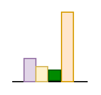
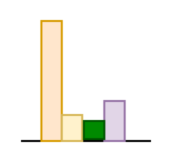
Exhaustively search for all possible sequences with the associated probabilities and output the sequence with the highest probability
I like cold water
I like cold coffee
coffee like cold coffee
coffee coffee coffee coffee
I like I like
I like cold coffee
p(\cdot)=0.15
coffee like cold coffee
p(\cdot)=0.1
I like I like
p(\cdot)=0.001
I like coffee
p(\cdot)=0.12
coffee coffee coffee coffee
p(\cdot)=0.0001
I like cold water
p(\cdot)=0.1
I like cold coffee
Outputs*
* Assuming the sequence has the highest probability among all \(|\mathcal{V}|^5\) sequences
Suppose that we want to generate a sequence of 5 words with the vocabulary \(\{ cold, coffee,I,like,water,<stop>\}\)
A
B
C
p(A|C)
p(B|C)
p(C|C)
p(A|B)
p(B|B)
p(C|B)
p(A|A)
p(B|A)
p(C|A)
t=1
t=2
max()

0.3
0.5
0.2
0.8
0.1
0.1
0.6
0.2
0.2
0.5
0.4
0.1
p(x_1,x_2)
Exhaustive search for a sequence of length 2 with the vocabulary of size 3
At time step-1, the decoder outputs probability for all 3 tokens
At time step-2, we need to run the decoder three times independently conditioned on all the three predictions from the previous time step
At time step-3 we will have to run the decoders 9 times
If \(|\mathcal{V}|=40000\), then we need to run the decoder 40000 times in parallel
Illustration
| 1 | 2 | 3 | 4 | 5 |
|---|---|---|---|---|
cold
<stop>
coffee
I
like
water
time steps
I
like
cold
coffee
<stop>
p(w_1=I)=0.4
At each time step, we always output the token with the highest probability (Greedy)
p(w_2=like|w_1=I)=0.35
p(w_3=cold|w_1,w_2)=0.45
p(w_4=coffee|w_1,w_2,w_3)=0.35
p(w_5=stop|w_1,w_2,w_3,w_4)=0.5
p(w_5,w_1,w_2,w_3,w_4)= \\
0.5 \times 0.35 \times 0.45 \times0.35 \times0.4= 0.011
0.1
0.15
0.25
0.4
0.05
0.05
0.1
0.15
0.25
0.05
0.35
0.1
0.45
0.05
0.1
0.05
0.15
0.2
0.15
0.3
0.35
0.01
0.09
0.1
0.1
0.5
0.2
0.1
0.05
0.05
Then the probability of the generated sequence is
Greedy Search
On the other extreme we can do a greedy search
| 1 | 2 | 3 | 4 | 5 |
|---|---|---|---|---|
cold
<stop>
coffee
I
like
water
time steps
I
like
cold
coffee
<stop>
p(w_5,w_1,w_2,w_3,w_4)= \\
0.5 \times 0.35 \times 0.45 \times0.35 \times0.4= 0.011
0.1
0.15
0.25
0.4
0.05
0.05
0.1
0.15
0.25
0.05
0.35
0.1
0.45
0.05
0.1
0.05
0.15
0.2
0.15
0.3
0.35
0.01
0.09
0.1
0.1
0.5
0.2
0.1
0.05
0.05
Then the probability of the generated sequence is
Is this the most likely sequence?
What if we picked the second most probable token in the first time step?
What if we want to get a variety of sequences of the same length?
Some Limitations
If the starting token is the word "I", then it will always end up producing the same sequence:I like cold coffee
we would have ended up with a different sequence.
| 1 | 2 | 3 | 4 | 5 |
|---|---|---|---|---|
cold
<stop>
coffee
I
like
water
time steps
coffee
like
cold
water
<stop>
p(w_5,w_1,w_2,w_3,w_4)= \\
0.5 \times 0.35 \times 0.45 \times0.35 \times0.4= 0.011
0.1
0.15
0.25
0.4
0.05
0.05
0.65
0.05
0.05
0.05
0.1
0.1
0.04
0.01
0.1
0.03
0.02
0.8
0.1
0.5
0.2
0.1
0.05
0.05
Then the probability of the generated sequence is
Then the conditional distribution in the subsequent time steps will change.
0.15
0.1
0.05
0.05
0.55
0.1
p(w_5,w_1,w_2,w_3,w_4)= \\
0.25 \times 0.55 \times 0.65 \times0.8 \times0.5= 0.035
Then the probability of the generated sequence is
Why not follow this at every time step?
We could output this sequence instead of the one generated by greedy search.
Greedily selecting a token with max probability at every time step does not always give the sequence with maximum probability
What if we picked the second most probable token in the first time step?
Beam Search
Instead of considering probability for all the tokens at every time step (as in exhaustive search), consider only top\(-k\) tokens
t=1
0.5
0.4
0.1
0.1
0.2
0.5
0.2
0.2
0.6
t=2
A
B
C
p(A|A)
p(B|A)
p(C|A)
p(A|B)
p(B|B)
p(C|B)
\times
\times
Now we have to choose the tokens that maximize the probability of the sequence
\times
\times
Suppose (\(k=2\))
p(A)p(A|A)=0.5 \times 0.1=0.05
p(A)p(B|A)=0.5 \times 0.2=0.01
p(A)p(C|A)=0.5 \times 0.5=0.25
p(B)p(A|B)=0.4 \times 0.2 =0.08
p(B)p(B|B) = 0.4 \times 0.2 =0.08
p(B)p(C|B) = 0.4 \times 0.6 =0.24
It requires \(k\times |\mathcal{V}|\) computations at each time step
Beam Search
Instead of considering probability for all the tokens at every time step (as in exhaustive search), consider only top\(-k\) tokens
t=1
0.5
0.4
0.1
0.1
0.2
0.5
0.2
0.2
0.6
t=2
0.55
0.25
0.2
t=3
A
B
C
p(A|A)
p(B|A)
p(C|A)
p(A|B)
p(B|B)
p(C|B)
0.1
0.75
0.15
p(B|C,A)
p(A|B,C)
P(A,C,B)=0.18
P(B,C,A)=0.13
0.25
0.24
Suppose (\(k=2\))
Following the similar calculations, we end up choosing
Over
Beam Search
Instead of considering probability for all the tokens at every time step (as in exhaustive search), consider only top\(-k\) tokens
t=1
0.5
0.4
0.1
0.1
0.2
0.5
0.2
0.2
0.6
t=2
0.55
0.25
0.2
t=3
A
B
C
p(A|A)
p(B|A)
p(C|A)
p(A|B)
p(B|B)
p(C|B)
The parameter \(k\) is called beam size. It is an approximation to exhaustive search.
If \(k=1\), then it is equal to greedy search.
Now we will have \(k\) sequences at the end of time step \(T\) and output the sequence which has the highest probability.
0.1
0.75
0.15
It is a better approximation to exhaustive search.
p(B|C,A)
p(A|B,C)
P(A,C,B)=0.18
P(B,C,A)=0.13
A
train
steam
engine
track
engine
the
is
oil
train
turbine
is
spilled
making
made
a
the
costly
available
noise
sound
\langle stop \rangle
at
Now backtrack
A \ train \ engine \ is \ making \ the \ noise
A \ train \ engine \ oil \ is \ costly
Output the sequence which has the highest probability
Divide the probability of the sequence by its length (otherwise longer sequences will have lower probability)

Neither greedy search nor beam search can result in creative outputs
Both the greedy search and the beam search are prone to be degenerative
Latency for greedy search is lower than beam search
Note however that the beam search strategy is highly suitable for tasks like translation and summarization
We are surprised when something is creative!
Surprise = uncertaininty
Sampling Strategies
Top-K sampling
At every time step, consider \(top-k\) tokens from the probability distirbution
| 1 | 2 | 3 | 4 | 5 |
|---|---|---|---|---|
cold
<stop>
coffee
I
like
water
time steps
0.1
0.15
0.25
0.4
0.05
0.05
0.65
0.05
0.05
0.05
0.09
0.11
0.04
0.01
0.1
0.03
0.02
0.8
0.1
0.5
0.2
0.1
0.05
0.05
0.1
0.15
0.05
0.05
0.55
0.1
Sample a token from the top-k tokens!
Say, \(k=2\)
Let's generate a sequence using Top-K sampling
I
<stop>
I
<stop>
or it could have produced
The proability of top-k tokens will be normalized relatively, \(P(I)=0.61,P(coffee)=0.39\) before sampling a token.
Top-K sampling
| 1 | 2 | 3 | 4 | 5 |
|---|---|---|---|---|
cold
<stop>
coffee
I
like
water
time steps
0.1
0.15
0.25
0.4
0.05
0.05
0.65
0.05
0.05
0.05
0.09
0.11
0.04
0.01
0.1
0.03
0.02
0.8
0.1
0.5
0.2
0.1
0.05
0.05
0.1
0.15
0.05
0.05
0.55
0.1
coffee
like
cold
coffee
<stop>
coffee
like
cold
coffee
<stop>
How does random sampling help?
At every time step, consider \(top-k\) tokens from the probability distirbution
Sample a token from the top-k tokens!
Say, \(k=2\)
Let's generate a sequence using Top-K sampling
I
<stop>
or it could have produced
Surprise is an outcome of being random
How does beam search compare with human prediction at every time step?

Human predictions have a high variance whereas beam search predictions have a low variance.
Giving a chance to other highly probable tokens leads to a variety in the generated sequences.

What should the optimal value of k be?
she
said
,
"
I
never
thought
knew
had
saw
said
could
meant
\vdots
If we fix the value of,say, \(k=5\), then we are missing out other equally probable tokens from the flat distribution.
It will miss to generate a variety of sentences (less creative)
I
ate
the
pizza
while
it
was
still
hot
cooling
warm
on
heating
going
For a peaked distribution, using the same value of \(k=5\), we might end up creating some meaning less sentences
as we are taking tokens that are less likely to come next.
Solution-1:Low temparature sampling
P(x=u_l|x_{1:i-1})=\frac{exp(\frac{u_l}{T})}{\sum_{l'} exp(\frac{u_{l'}}{T})}
Given the logits, \(u_{1:|V|}\), and temperature parameter \(T\), compute the probabilities as
Low temperature = skewed distribution = less creativity
high temperature = flatter distribution = more creativity
Solution:2 Top-P (Nucleus) sampling
Set a value for the parameter \(p, \ 0<p<1\).
Sum the probabilities of tokens starting from the top token.
Sort the probabilities in descending order
If the sum exceeds \(p\), then sample a token from the selected tokens.
It is similar to \(top-k\) with \(k\) being dynamic.
she
said
,
"
I
never
thought
knew
had
saw
said
could
meant
\vdots
I
ate
the
pizza
while
it
was
still
hot
cooling
warm
on
heating
going
Suppose we set \(p=0.6\),
For top left distribution: the model will sample from the tokens (thought,knew,had,saw,said)
For bottom left distribution: the model will sample from the tokens (hot,cooling)
Speculative Decoding/Assisted Generation
The various approaches that we have discussed so far was focusing on generating diverse and quality sentences but not on reducing the time complexity (or latency)
All tokens are generated sequentially in autoregressive sampling. Therefore, the time complexity to generate \(N\) tokens is \(O(N \cdot t_{model})\)
That's what the speculative decoding strategy try to address
It becomes a significant performance bottleneck for larger models.
Assigning 1 byte of memory requires 530GB of GPU memory
Assume a larger language model with 500+ Billion parameters.
This requires us to distribute the model across multiple GPUs (Model parallelism) that adds additional communication overhead to the final latency
To generate a single token, we need to carryout at least 500+ Billion operations
How? Let's see
(somehow) Parallelizing the process reduce the latency
Moreover, the sampling process is sequential
Rejection Sampling
Suppose we want to sample \(\tilde{x}\) from a complex distribution \(q(x)\) called target distribution.
Instead of directly sampling from the complex distribution \(q(x)\), we sample \(\tilde{x}\) from a simple distribution \(p(x)\) called draft distribution.
We accept or reject the sample \(\tilde{x}\) based on the following rule
\mathbb{I}=\frac{q(\tilde{x})}{c*p(\tilde{x})}>r
where \(\mathbb{I} \in \{0,1\}\) is an indicator variable and \(r \sim U(0,1)\) and \(c\) is a constant. The sample is accepted if \(\mathbb{I}=1\).
Note that a lot of samples got rejected!
Out of 100 samples, only 15 were accepted. The efficiency is 0.15 percent!
Increasing efficiency requires us to assume reasonably better draft distribution!
Draft Model \(q(.|.)\)
7B parameters
We Apply the same idea here
Use a smaller but faster model (called draft model) that speculates (lookahead) \(K\) future(candidate) tokens in the Auto-Regressive manner
The more you learn
the
k=4

more
you
can
do
Draft Model \(p(.|.)\)
7B parameters
We Apply the same idea here
Use a smaller but faster model (called draft model) that speculates (lookahead) \(K\) future(candidate) tokens in the Auto-Regressive manner
k=5
p(x|x_1,\cdots,x_4)=argmax(p(.|.))=the
Using greedy search (for ex)
p(x|x_1,\cdots,x_4,x_5)=more
p(x|x_1,\cdots,x_4,x_5,x_6)=you
p(x|x_1,\cdots,x_4,x_5,x_6,x_7)=can
The more you learn
the
more
you
can
do
p(x|x_1,\cdots,x_4,x_5,x_6,x_7,x_8)=do
Target \(q(.|.)\)
70 B parameters
Use a larget but slower model (called target model) that accepts or rejectis a subset of \(K\) tokens using some rejection criteria.
k=5+1
q(x=the|x_1,\cdots,x_4)
In Parallel, compute
q(x=more|x_1,\cdots,x_4,x_5)
q(x=you|x_1,\cdots,x_4,x_5,x_6)
q(x=can|x_1,\cdots,x_4,x_5,x_6,x_7)
The more you learn
q(the)
q(more)
q(you)
q(can)
q(do)
q(x=do|x_1,\cdots,x_4,x_5,x_6,x_7,x_8)
The more you learn the
The more you learn the more
The more you learn the more you can
The more you learn the more you can do
q(.)
Accept-Reject criterion
Now we have probabilities from both draft \(p(.|.)\) and target \(q(.|.)\)models.
Remember that the propablities for the \(K\) tokens were computed in parallel by the target \(q(.|.)\)model.
for \(t=1:K\):
sample \(r \sim U(0,1)\)
if \(r < min\big(1,\frac{q(x|x_1,\cdots,x_{n+t-1})}{p(x|x_1,\cdots,x_{n+t-1})}\big)\):
Accept the token: \(x_{n+t} \leftarrow x\)
else:
Resample from modified distribution
\(x_{n+t} \sim (q(x|x_1,\cdots,x_{n+t-1}) - p(x|x_1,\cdots,x_{n+t-1}))_+\)
exit for loop
If all tokens are accepted, sample \(K+1\)th token from \(q(.|.)\)
(f(x))_+= \frac{max(0,f(x))}{\sum_x max(0,f(x))}
What have we gained by Speculative Decoding?
At each iteration, it predicts atleast 1 (if all rejected) to atmost \(K+1\) tokens (if all accepted).
It reduces the time complexity from \(O(N \cdot t_{target}) \) to the best case of \(O(\frac{N}{K+1} \cdot (Kt_{draft}+t_{target}) \)
Contrastive Decoding
Expert Model
GPT-XL
Amateur Model
GPT-small
Barack Obama was born in Honolulu, Hawai. He was born in
| 0.27 | Hawaii |
| 0.18 | the |
| 0.16 | Honolulu |
| 0.10 | 1961 |
| 0.02 | Washington |
| 0.08 | Honolulu |
| 0.04 | washington |
| 0.04 | the |
| 0.001 | 1961 |
P_{exp}
P_{axp}
Prompt
Greedy search
Barack Obama was born in Honolulu, Hawai. He was born in Hawai
Top-k/Top-p
Barack Obama was born in Honolulu, Hawai. He was born in Washington
We are facing a problem of repetition and incoherence!
Consider only plausible tokens from the expert model using plausibility constraint.
Contrastive Decoding
Expert Model
GPT-XL
Amateur Model
GPT-small
Barack Obama was born in Honolulu, Hawai. He was born in
| 0.27 | Hawaii |
| 0.18 | the |
| 0.16 | Honolulu |
| 0.10 | 1961 |
| 0.02 | Washington |
| 0.08 | Honolulu |
| 0.04 | washington |
| 0.04 | the |
| 0.001 | 1961 |
log_{P_{exp}}-log_{P_{ama}}
P_{exp}
P_{axp}
| 4.6 | 1961 |
| 2.34 | Hawaii |
| 0.65 | Honolulu |
| -0.73 | Washington |
Contrastive Decoding
Prompt
Barack Obama was born in Honolulu, Hawai. He was born in 1961
References
References
Controlled text generation summary: https://lilianweng.github.io/posts/2021-01-02-controllable-text-generation/
IntrotoGPT-Decoding-Strategies
By Arun Prakash


