Introduction to Large Language Models
Handling Long Sequences, Computational Complexity of Transformers, Fast Attention Mechanisms
Mitesh M. Khapra, Arun Prakash A


AI4Bharat, Department of Computer Science and Engineering, IIT Madras
Motivation
The models that we have discussed so far have a limited context length of 512 or 1024(GPT-2)
What about other sequences like audio and images (viewing pixels as sequences)?
The sequence length of an audio signal of 10s duration is about 80000 (assuming sampling rate of 8000 Hz)
The sequence length of a colour image of size 100 by 100 is 30000.
So, enabling the models to attend to longer sequences is crucial.
What if we want to summarize a book that contains, say 64000 words?
What if we want to generate a story that contains at least 5000 words?
What if we want to find an answer to a question from an instruction manual that contains a thousand pages?
Motivation
The context lengths of some of the recent models are listed below
| Model | Context length |
|---|---|
| LLAMA-2 | 4K |
| Mistral-7B | 8K |
| GPT-4, Gemini 1.0 | 32K |
| Mosaic ML MPT | 65K |
| Anthropic Claude | 100K |
| Gemini 1.5 pro, GPT-4 Turbo | 128K |
| Claude 2.1 | 200K |
| Gemini 1.5 pro (limited) | 2 million (for public) 10 million (experimental) |
Why is it difficult to scale the context length?
One of the primary factors is the computational complexity of the self-attention mechanism.
Let us first try to understand the computational complexity and memory requirements to train Transformer based models.
Module 1: Time and Space Complexity of Attention Mechanism
AI4Bharat, Department of Computer Science and Engineering, IIT Madras
Mitesh M. Khapra, Arun Prakash A
Attention Mechanism
T
d
d
T
Q
K^T
Context window size: \(T\)
The size of the (projected) embeddings: \(d = d_q=d_k\)
Attention Mechanism
T
d
d
T
Q
K^T
Context window size: \(T\)
The size of the (projected) embeddings: \(d = d_q=d_k\)
One dot product between \(d_q \cdot d_k^T\) requires \(d\) multiplications and \(d-1\) additions
Attention Mechanism
T
d
d
T
Q
K^T
Context window size: \(T\)
The size of the (projected) embeddings: \(d = d_q=d_k\)
Number of operations for computing one row of unnormalized attention weights \(Z \in \mathbb{R}^{T \times T}\) is..
\(T \cdot d\) multiplications and \(T \cdot (d-1)\) additions
Attention Mechanism
T
d_q
d_k
T
Q
K^T
Context window size: \(T\)
The size of the (projected) embeddings: \(d = d_q=d_k\)
Number of operations for computing one row of unnormalized attention weights \(Z \in \mathbb{R}^{T \times T}\) is:
\(T \cdot d\) multiplications and \(T \cdot (d-1)\) additions
The number of tokens \(T\) is typically greater than embedding dimension \(d\).
Therefore, to compute \(QK^T\) we require \(\mathcal{O}(T^2d)\) operations
What about computing attention score by normalizing the unnormalized matrix \(Z\) ?
Q
K^T
Attention Mechanism
T
d_q
d_k
T
Q
K^T
Q
K^T
T
T
A=softmax(\frac{QK^T}{\sqrt{d}})
There are \(T\) rows in \(Z\), therefore computational complexity for \(softmax\) is \(\mathcal{O}(T^2)\).
\(\therefore\) The computational complexity of \(A\) is \(\mathcal{O}(T^2d)\).
We need to normalize each row of \(Z\), this requires \(O(T)\) operations.
Z
Attention Mechanism
T
T
A
V
d
T
Finally, the attention score matrix \(A\) is multiplied with the value matrix \(V\)
Attention Mechanism
T
T
A
V
d
T
Therefore, the entire self-attention block is quadratic \(\mathcal{O}(T^2d)\) in the length of the input sequence.
Finally, the attention score matrix \(A\) is multiplied with the value matrix \(V\)
This has a complexity of \(O(T^2 d)\)
Attention Mechanism
T
T
A
V
d
T
Therefore, the entire self-attention block is quadratic \(\mathcal{O}(T^2d)\) in the length of the input sequence.
Finally, the attention score matrix \(A\) is multiplied with the value matrix \(V\)
This has a complexity of \(O(T^2 d)\)
Module 2: Memory Requirements
AI4Bharat, Department of Computer Science and Engineering, IIT Madras
Mitesh M. Khapra, Arun Prakash A
Notations
\(B\): Batch Size

B
d_{model}
T
\(T\) : Context (sequence) Length
\(n_h\) : Number of attention heads
\(d_{model}\) : Dimension of input embedding, \(d_{att}=512=\frac{d_{ff}}{4}\)
\(N\) : Number of parameters in the model
\(|\mathcal{V}|\) : Number of tokens in the vocabulary
\(d_{ff}\) : Dimension of feed-forward layer
Total Memory required is the sum of memory for
Storing Activation values
Storing Parameters
Storing Gradients
Which of these do you think takes the most memory?
Memory for Attention
mha= (Q_{T \times d}+K_{d \times T}^T + V_{T \times d}) n_h
=3BTd_{model}
= 3n_h(T\times d)
= 3T\times n_h d
= 3T\times d_{model} \quad \because n_hd=d_{model}
A= softmax(QK^T)
Z = QK^T
=Bn_hT^2
=Bn_hT^2
Memory scales up linearly with respect to batch size \(B\) and quadratically with respect to the length of the context window \(T\).
For a single sample
For a batch of \(B\) samples
Key Take Aways
The complexity of Self-attention is quadratic in the length of the input sequence.
Memory scales up linearly with respect to batch size \(B\) and quadratically with respect to the length of the context window \(T\).
So, the next question is, How do we reduce the time complexity to enable models to handle long sequences (during both training and inference)?
Module 3: Fast Attention Mechanisms
AI4Bharat, Department of Computer Science and Engineering, IIT Madras
Mitesh M. Khapra, Arun Prakash A
What we have is the full attention mechanism with \(O(T^2d)\) complexity. What we want is sub-quadratic complexity \(O(cTd)\). How do we achieve that?
Objective
Well, we can localize the attention in multiple ways.
This gives rise to a plethora of approaches that approximate the full attention.
O(T^2d)
A study on BERT [Ref] in NLP tasks concluded that the neighbouring inner products are extremely important in self-attention and not all heads attend to all tokens.

Approaches
O(T^2d)
Strided Local Attention
O(T^2d)
Strided Local Attention
Approaches
Random Local Attention
O(T^2d)
Sparse Block Attention
Strided Local Attention
Approaches
Random Local Attention
O(T^2d)
Sparse Block Attention
Strided Local Attention
Global+local attention
Approaches
Random Local Attention
Sparse Block Attention
Strided Local Attention
Global+local attention
Random Local Attention
Approaches
O(T^2d)
Flash Attention
Our planet is a lonely speck
Full Attention
Every word attends to every other word in the input sequence
Our planet is a lonely speck
\vdots
Our planet is a lonely speck
Computational complexity \(O(T^2d)\)
How do we reduce the computational complexity?
Our focus is on reducing the computational complexity.
Memory complexity \(O(T^2)\)
One way is to make it sparse by attending to a subset of words instead of all words
(the score for the word itself (\(q_ik_i^T\)))
QK^T
\(O(c \times T \times d)\) where \(c < T\)
Our planet is a lonely speck
Strided Local Attention
Our planet is a lonely speck
\vdots
Our planet is a lonely speck
Linear Computational complexity \(O(cTd)\)
QK^T
\(c=3\)
Every word attends to a window of \(c\) words (\(\lfloor \frac{c}{2} \rfloor\) to the left and \(\lfloor \frac{c}{2} \rfloor\) words to the right)
We could vary the size of the window for each layer in the model such that the top most layer uses the full (global) attention
Strided Local Attention
\(O(3Td)\)
QK^T
\(c=3\)
QK^T
\(c=5\)
\(O(5Td)\)
Our planet is a lonely speck
Our planet is a lonely speck
\vdots
Our planet is a lonely speck
Every word attends to a window of \(c\) words (\(\lfloor \frac{c}{2} \rfloor\) to the left and \(\lfloor \frac{c}{2} \rfloor\) words to the right)
Our planet is a lonely speck
Our planet is a lonely speck
\vdots
Our planet is a lonely speck
We could also use dilated attention (like dilated convolutions) by using different dilation rates in different attention heads.
Dilated Attention
\(O(3Td)\)
QK^T
\(c=3\)
Note that, there is no change in computational complexity.
Every word attends to a window of \(c\) words (\(\lfloor \frac{c}{2} \rfloor\) to the left and \(\lfloor \frac{c}{2} \rfloor\) words to the right)
Tokens like [cls] requires full attention to get good performance in downstream tasks.
Global + local Attention
\(O((3T+T)d)\)
QK^T
\(c=3\)
[cls] Our planet is a lonely speck
We can manually set tokens that require global attention based on the task.
A few words are global, every other word attends to a window of \(c\) words (\(\lfloor \frac{c}{2} \rfloor\) to the left and \(\lfloor \frac{c}{2} \rfloor\) words to the right).
Our planet is a lonely speck
Our planet is a lonely speck
\vdots
Our planet is a lonely speck
Tokens like [cls] requires full attention to get a good performance in downstream tasks.
Global + Random+ local Attention
\(O((3T+T+T)d)\)
QK^T
\(c=3\)
[cls] Our planet is a lonely speck
The BIGBIRD model proposes adding random tokens.
A few words are global, every other word attends to a window of \(c\) words (\(\lfloor \frac{c}{2} \rfloor\) to the left and \(\lfloor \frac{c}{2} \rfloor\) words to the right).
Our planet is a lonely speck
Our planet is a lonely speck
\vdots
Our planet is a lonely speck
Our planet is a lonely speck
Local Block Attention
Another way is to divide the sequence into \(n\) blocks and do the computations independently as in [Ref]
Computational complexity \(O(\frac{T^2}{2})\)
QK^T
Typically, \(n=2,3,4\). Therefore, for a context length of 512, the block sizes will be 256, 128, 64.
These are resonable context sizes for majority of NLP tasks.
MHA
MHA
Merge
We could also use different patterns in each attention head/layer.
Suppose we have \(n=4\) blocks. Then we can permute these blocks in 16 possible ways (how? will see soon)
Therefore, we can permute these blocks in each attention head so that it could effectively capture long range dependencies.
Full Attention
Q \in \mathbb{R}^{T\times d_k}
K \in \mathbb{R}^{d_k\times T}
QK^T \in \mathbb{R}^{T\times T}
Let's recall how we compute the attention matrix
Full Attention
Q \in \mathbb{R}^{T\times d_k}
K \in \mathbb{R}^{d_k\times T}
QK^T \in \mathbb{R}^{T\times T}
Q_0
Q_1
Q_2
K_0^T
K_1^T
K_2^T
Q_0K_0^T
Q_0K_2^T
Q_2K_2^T
Let's recall how we compute the attention matrix.
We can divide \(Q\) and \(K\) matrices into \(n\) blocks each. This will result in \(n^2\) blocks in \(QK^T\) as shown in the figure above.
Block Attention
Q \in \mathbb{R}^{T\times d_k}
K \in \mathbb{R}^{d_k\times T}
QK^T \in \mathbb{R}^{T\times T}
Q_0
Q_1
Q_2
K_0^T
K_1^T
K_2^T
Q_0K_0^T
Q_1K_2^T
Q_2K_1^T
V_0
V_1
V_2
Let's recall how we compute the attention matrix.
We can divide \(Q\) and \(K\) matrices into \(n\) blocks each. This will result in \(n^2\) blocks in \(QK^T\) as shown in the figure above.
Suppose we want to select only 3 blocks.
Q \in \mathbb{R}^{T\times d_k}
K \in \mathbb{R}^{d_k\times T}
QK^T \in \mathbb{R}^{T\times T}
Q_0
Q_1
Q_2
K_0^T
K_1^T
K_2^T
Q_0K_0^T
Q_1K_1^T
Q_2K_2^T
V_0
V_1
V_2
There are many ways of selecting 3 blocks from the set of \(B=9\) blocks. Let's formalize this.
Suppose we want to select only 3 blocks.
Let's recall how we compute the attention matrix
We can divide the each \(Q\) and \(K\) matrices into \(n\) blocks, this will result in \(n^2\) blocks in \(QK^T\) as shown in the figure above
Block Attention
Block Attention
Z = softmax(QK^T \odot M)
M_{ij}=\begin{cases}1 & \text{if} \quad \pi(\lfloor\frac{in}{T}\rfloor)=\lfloor\frac{jn}{T}\rfloor \\
0 & \text{otherwise}
\end{cases}

\pi = (0,1,2)
\pi = (0,2,1)
Block Attention is given by,
For example, suppose context length \(T=15\) and the number of blocks \(n=3\).
Write \(Q\),\(K^T\), and \(V\) into \(n=3\) block matrices (following the blocks in \(M\))
\textbf{Q}=(Q_0,Q_1,Q_2) \in \mathbb{R}^{5 \times d}
\textbf{K}=(K_{\pi(0)},K_{\pi(1)},K_{\pi(2)})\in \mathbb{R}^{5 \times d}
\textbf{V}=(V_{\pi(0)},V_{\pi(1)},V_{\pi(2)}) \in \mathbb{R}^{5 \times d}
Then we would have 3! ways of permuting the blocks.
Consider the permutation,
\(\pi=\text{perm}(0,1,2,\cdots, n-1)\)
Let the \(k\)-th element of \(\pi\) be \(\pi(k)\), We define the masking matrix \(M\) of size \(T \times T\)
n = 3, T = 15
n = 3, T = 15
Identity:
Computational Complexity
Using these we can compute Block Attention as follows
\text{Block-wise Attention}(Q,K,V,M)
=\begin{bmatrix}
softmax(Q_0K_{\pi(0)}^T)V_{\pi(0)} \\ \vdots \\
softmax(Q_nK_{\pi(n-1)}^T)V_{\pi(n-1)}
\end{bmatrix}
\frac{T}{n} \times \frac{T}{n} \times d
=O\big(\frac{T}{n} \times \frac{T}{n}
\times n \times d \big)
\frac{T}{n} \times \frac{T}{n} \times d
=O\big(\frac{T^2d}{n}\big)
We can extend the same concept to Multi-head attention by allowing each head to use a different masking matrix (derived from the permutation function).
This would be called Blockwise Multi-Head Attention.
What happens if we increase value of \(n\)?

T=32, n=2
T=32, n=16
50% non-zero values

Identity:(0,1)
(8, 5, 15, 4, 7, 10, 11, 2, 3, 1, 12, 13, 9, 6, 14, 0)
6.25% non-zero values
(50% sparse)
(93% sparse)
Capturing Long Term dependency
Blockwise sparsity captures both local and long-distance dependencies in a memory-efficient way using different permutations

Empirically, it is observed that the identity permutation is more important than other permutations

Using blockwise sparse attention reduces the training time significantly for longer sequences.
Note, however, that the perplexity score increases as the number of blocks \(n\) increases.
This is reasonable given that local attention is just an approximation to full attention. (This is the case for all local attention schemes.)
Performance
Locality Sensitive Hashing [Paper]

Let us pick up two rows in the attention matrix show on the left
For the given query \(q_i\), we know that the attention score is higher for some of the keys \(k_j\)
Can we find those \(k_j\)'s without resorting to computing pair-wise dot product with all the keys?
It is similar to approximating attention using the K-Nearest Neighbours (KNN) search. For example, if K is of length 64K, for each \(q_i\) we could only consider a small subset of, say, the 32 or 64 closest keys
One of many possible ways of doing this is to use Locality Sensitive Hashing (LSH) (Yes, the same one we used for deduplication of contents!)
The attention matrix is mostly sparse !
However, there is a catch!
For this to work, we need \(Q=K\).This requires us to share the weight matrices \(W_Q=W_K\).
We look for a hashing scheme that assigns each vector \(x\) (query) to a hash bucket such that nearby vectors falls in the same hash bucket and distant ones do not. This is called locality-sensitive hashing
Let's see how we construct hash buckets using a hash function with a help of an example (in 2D case)

h(x)

\in \mathbb{R}^{d}
\in \mathbb{R}^{d}
For each query, it takes \(log(T)\) time to find the approximate nearest neighbours [ref], therefore, its computational complexity is \(O(T \log(T))\)
Assume,
d_k = dq = 64
Consider a query (and a key) \((x=q_1,y=k_2)\) that are away from each other and first projected onto a sphere
q_1,k_2\in \mathbb{R}^{1 \times 64}
Define the number of hash buckets, \((b=4)\)
Let the random rotation matrix \(R\) be of size \([d_k,b/2]\).
hash(x)= \textit{argmax}(concat(xR,-xR))
for illustration,
R \in \mathbb{R}^{64 \times 2}
Let us define the hash function

0
1
2
3
\(hash(q_1)= \textit{argmax}(concat(0.5,0.25,-0.5,-0.25))=0\)
\(hash(k_2)= \textit{argmax}(concat(-0.25,-0.5,0.25,0.5))=3\)
\(hash(q_1)= \textit{argmax}(concat(0.5,0.25,-0.5,-0.25))=0\)
\(hash(k_2)= \textit{argmax}(concat(-0.25,-0.5,0.25,0.5))=3\)
Recompute the hash by changing the rotation matrix a few times


The probability that the given query and the key share the same bucket is \(\frac{1}{3}\). Therefore, they are not close to each other
q_1:0 \quad \blue{2} \quad 1
k_2:3 \quad \blue{2} \quad 0
Let's consider a query and a key that are close to each other
Recompute the hash by changing the rotation matrix few times
The probability that the queries share the same bucket is \(\frac{3}{3}\). Therefore, they are close to each other
q_1:0 \quad \blue{2} \quad 1
k_2:0 \quad \blue{2} \quad 1

Therefore, all the points that are close to each other would share the same bucket.
Essentially compute the hash for all the queries (repeat \(n_R\) times if required)
This can be computed in parallel by multiplying all the queries with the random matrix \(R\)
| Query | hash by R1 | hash by R2 |
|---|---|---|
| 0 | 2 | |
| 3 | 2 | |
| 0 | 2 | |
| 0 | 2 |
q_1
q_2
q_3
q_{16}
\vdots
\vdots
\vdots
Now, sort the queries by bucket number,
Essentially compute the hash for all the queries (repeat \(n_R\) times if required)
This can be computed in parallel by multiplying all the queries with the random matrix \(R\)
| Query | hash by R1 | hash by R2 |
|---|---|---|
| 0 | 2 | |
| 0 | 2 | |
| 0 | 2 | |
| 3 | 2 |
q_1
q_2
q_3
q_{16}
\vdots
\vdots
\vdots
Now, sort the queries by bucket number,
Compute the attention scores for queries within each bucket. For example, in ClM, \(q_3 \) attends to \(q_1\), and \(q_{16}\) attends to \(q_3\) and \(q_{1}\) and so on
and within each bucket, by sequence position
The entire procedure is captured in the figure below

The entire procedure is captured in the figure below
The entire procedure is captured in the figure below
The entire procedure is captured in the figure below
The entire procedure is captured in the figure below
Self-attention is Low rank [paper]
The methods that we have seen so far localize or sparsify the attention matrix in different ways
The theoretical time complexity is sub-quadratic \(O(cTd)\), with \(c\) being a constant (manually set, or function of \(T\) such as \(log(T)\))
Can we reduce it to \(O(Td)\)? Yes, as follows :-)
Well, this is not helpful to capture the context.
However, we can see from empirical observation that the self-attention matrix is essentially low-rank (especially for the top layers)!
Apply SVD on the matrix \(A\) across different layers and different heads of the model, and plot the normalized cumulative singular value averaged over 10k sentences.
A=softmax(\frac{QK^T}{\sqrt{d}})
Consider a RoBERTa model trained on Wiki-103 (MLM task) and a classification task.
A \in \mathbb{R}^{512 \times 512}
Suppose we plot the distribution of all 512 singular values . Then, for it to be a low-rank it should follow a ____ distribution.
They observed a long tail distribution. Hence they concluded the matrix A is a low-rank matrix.

Using this observation, they show that there exists a low-rank approximation of \(QK^T\) and we can let the network to find (learn) it! How?
Q \in \mathbb{R}^{T \times d}
K \in \mathbb{R}^{T \times d}
V \in \mathbb{R}^{T \times d}
Introduce two learnable linear projection matrices
E,F \in \mathbb{R}^{k \times T}
A=softmax(\frac{Q(EK)^T}{\sqrt{d}})
O=AFV
A \in \mathbb{R}^{T \times k}

Q
K
V
The computational complexity is \(O(kTd)\), where \(k\) is the rank and can be set according to the error \(\epsilon\)
Kernel Methods [paper]
All that we need is an attention matrix such that each row sums up to one
Atten=softmax(\frac{QK^T}{\sqrt{d}})
Fundamentally, the exponential function in \(A\) takes in the query and key vectors and outputs a positive number.
A(i,j)=SM(q_i,k_j)=\mathcal{K}(q_i,k_j))
Atten=D^{-1}A
where,
A=exp(QK^T/\sqrt{d})
D=diag(A\mathbf{1})
\(\mathbf{1}\) is a vector of all ones of length \(T\)
So we can generalize this
\mathcal{K}:\mathbb{R}^d \times \mathbb{R}^d \to \mathbb{R}_+
\(\mathcal{K}\) is called a Kernel function, and defined as follows
\mathcal{K}(q_i,k_j)=\mathbb{E}(\phi(q_i)^T\phi(k_j))
\phi(x):\mathbb{R}^d \to \mathbb{R}_+^r,r>0
Where \(\phi(x)\) is some randomized feature mapping and \(\mathbb{E}\) is an expectation operator.
Note that \(r>0\), and it is not necessary that \(r <d\).
For example, \(T=64k,d=4k\), then \(r=8k\) is also reasonable
How do we compute \(\phi(x)\)?
\phi(x):\mathbb{R}^d \to \mathbb{R}_+^r
\phi(x)=\frac{h(x)}{\sqrt{r}}\bigg(f_1(w_1^Tx),\cdots,f_1(w_r^Tx), \cdots, f_l(w_1^Tx),\cdots,f_l(w_r^Tx) \bigg)
The generalized form of a kernel transformation is given by,
f_1,f_2,\cdots,f_l: \mathbb{R} \rightarrow \mathbb{R}
w_1,\cdots,w_r: \mathbb{R^d}
where \(w_i\) is sampled from \(\mathcal{N}(\mathbf{0}_d,\mathbf{ I}_d)\)
\(w_i^Tx\) is a random projection, that is, the vector \(x\) is projected in a random direction given by \(w_i\) vector.
We can construct a random feature vector of size \(r\) by setting \(l=1\), considering \(f_1=exp\) and \(h(x)=exp(\frac{-||x||^2}{2})\) (Note, this particular setting is theoretically motivated among many possible choices.)
where,
\phi(x)=\frac{exp(\frac{-||x||^2}{2})}{\sqrt{r}}\bigg(exp(w_1^Tx),\cdots,exp(w_r^Tx)\bigg)
\phi(X)=\frac{1}{\sqrt{r}}exp\bigg(\mathbf{W}^TX-\frac{||X||^2}{2}\bigg)
Therefore,
where \(\mathbf{W} \in \mathbb{R}^{d \times r}\) ,\(X \in \mathbb{R}^{d \times T}\) and \(||X||^2\) is the \(L2-\)norm of column vectors in \(X\).
\(w_i \sim \mathcal{N}(\mathbf{0}_d,\mathbf{ I}_d)\)
We can collect all \(w_i\)s in a matrix \(\mathbf{W}\)
For all the queries \(q_i\)s in \(Q\), we can compute \(Q'\) as follows
Q'=\frac{1}{\sqrt{r}}exp\bigg(\mathbf{QW^T}-\frac{||Q||^2}{2}\bigg)
here, \(\mathbf{W} \in \mathbb{R}^{r \times d}\) ,\(Q \in \mathbb{R}^{T \times d}\) and \(||Q||^2\) is the \(L2-\)norm of row vectors in \(Q\).
Q' \in \mathbb{R}^{T \times r}
Similary, we can compute \(K' \in \mathbf{R}^{T \times r}\).
The \(\mathbf{W}\) matrix is orthogonalized using Gram-Schmidt orthogonalization procedure.
Orthogonalization of W helps reduce the variance of the softmax estimator for any dimensionality of \(d\). This requires \( r \leq d\).


The time complexity is \(O(rTd)\).
The approximated attention matrix for the given query and key is given by
\hat{A}(i,j) = \hat{SM}(q_i,k_j)= \frac{1}{r}
exp(q_i\mathbf{W}^T-\frac{||q_i||^2}{2})
exp(k_j\mathbf{W}^T-\frac{||k_j||^2}{2})^T
\hat{A}=Q'K'^T
and the vectorized version is given by
\(L=T\) in the figure below
All these approaches that we have discussed so far approximated the full attention.
Reduced FLOPS != Reduced Wall clock speed
However, it does not translate to wall-clock speed-up!
That is, suppose we train a model with the compute requirement \(C \propto T^2\) FLOPS for a day.
Reducing the compute requirement \(C \propto \frac{T^2}{2}\) FLOPS will not reduce the training time to half a day
So, the problem is not in the algorithm but..
Module 4: Know your hardware to get wall-clock speed
AI4Bharat, Department of Computer Science and Engineering, IIT Madras
Mitesh M. Khapra, Arun Prakash A
Flash Attention: Exact Attention with IO Awarness
All Transformer based language models are trained on GPUs.
However, it was observed that the implementation of MHA did not efficiently utilize GPUs.
In fact, the training time is now memory bound not compute bound!
Let us try to understand this with a help of a simple example.
What are the sequence of steps involved in computing any mathematical operation? For example, consider a product of two numbers and computing square root of the result
c=ab \\
d = \sqrt{c}
Main Memory (DRAM)
Compute
(Registers)
Read (a,b, and mul instruction)
write (c)
c=ab
Main Memory (DRAM)
Compute
(Registers)
Read (c, and sqrt instruction)
write (d)
Therefore, there are two read operations, two write operations and two compute operations. The compute was not utilized during writing the result back to memory!
Typically, after executing an operation, the result is written back to main memory.
How do we skip this redundant reading from/ writing to memory as we are aware that the result \(c\) will be used in the subsequent operation?
compute is idle
d = \sqrt{c}
Kernel fusion
We can fuse the sequence of operation (called kernel fusion) as follows \(c=\sqrt{ab}\)
Main Memory (DRAM)
Compute
(Registers)
Read (a,b, mul,sqrt)
write (c)
We can store the intermediate result of the multiply operation in the registers/cache memory and take square root on it, then write the final result back to main memory
Therefore, Kernel fusion helps optimally utilize the compute capacity by making it aware that the intermediate results need not be written back to main memory!
Let us see the amount of time spent by the naive implementation of MHA and MHA using Kernel fusion.
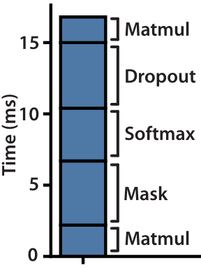
Naive implementation
Do you see anything surprising from the diagram?
Dropout, softmax, and masking take more time to execute than MatMul!
QK^T
QK^T+M
softmax(QK^T+M)
drop(softmax(QK^T+M))
drop(softmax(QK^T+M))V
In general, all element-wise operations like activation, normalization are all memory bound
A general approach to alleviate this problem is to use kernel fusion!
We write the output back to memory at every step and read the previous output as an input for the next step!
Naive implementation
QK^T
QK^T+M
softmax(QK^T+M)
drop(softmax(QK^T+M))
drop(softmax(QK^T+M))V
At every step, we write an output back to memory and read the previous output as an input for the next step!

There is a catch! We need to store \(QK^T\) for backward pass!
S=QK^T
P=Softmax(S)
O=PV
Getting into Details

Standard attention is memory bound.
Objective: Given \(Q,K,V\), compute \(O\) and write it to HBM (High Bandwidth Memory) (Note: using only one write operation).
We can not use entire Q, K, and V matrices. We need to divide each of these into blocks. Why?

Memory Hierarchy
High Bandwidth Memory (the one you get when you type nvidia-smi command) is the place where we load and store data, model parameters, and all intermediate results.
SRAM has small memory (20MB) (distributed across cores each of size about 100KB) with a high bandwidth (19TB/s)
Suppose we have a sequence of length 1024, to store \(Q,K\) using 4 bytes (32 bit) per element requires \(2 \times 1024 \times 64 \times 4 = 524 KB \).
So, it is not possible to fit in the entire Q and K matrices into SRAM.
IDEA
1. Tiling: Divide the matrices \(Q,K,V\) into small blocks (in HBM) such that it fits into the SRAM of size \(M\) (around 100 KB) and compute attention by blocks
Q_0
Q_1
Q_2
K_0^T
K_1^T
K_2^T
Q_0K_0^T
Q_0K_2^T
Q_2K_2^T
We apply the softmax function for each block of \(Q_iK_j^T\).
However, we have only \(S_{ij}\) but the softmax requires all the elements in \(S\) for normalization
S_{ij}=Q_iK_j^T
P=Softmax(S)
How do we go from \(S_{ij}\)'s to \(P\)?
IDEA
1. Divide the matrices \(Q, K,\) and \(V\) into small blocks (in HBM) such that it fits into the SRAM of size \(M\) (around 100 KB)
Q_0K_0^T
Q_0K_2^T
Q_2K_2^T
S_{ij}=Q_iK_j^T
f_{00}
f_{02}
f_{22}
\(P=ConCat(\beta_0f_{00},\beta_1f_{01},\cdots, \beta_8 f_{22}\))
(Q_iK_j^T).softmax()
\cdots
\cdots
\cdots
\cdots
How do we compute the weight \(\beta_i\) for each block ?
\(f_{ij}\) is an intermediate sequence
IDEA
How do we compute \(\beta_i\)?
Let us take a simple example to illustrate the idea
Before going further, we use a variation of softmax implementation called "Safe softmax" in which we subtract the maximum of the vector from all its elements because the exponential operator is more accurate for negative inputs [Ref]
\frac{e^{x_i}}{\sum \limits_j e^{x_j}}=
\frac{e^{x_i-m}}{\sum \limits_j e^{x_j-m}}
m=max(x)
where,
\(x=[x^A,x^B]\) where,\(x^A\): -1.02 -1.09 0.24 0.87 -1.32, \(x^B\): -0.6 -5.04 -2. 1.03 -0.14
Consider an example sequence \(x\) divided into two consecutive sub-sequences \(x^A\) and \(x^B\).
Online softmax
How do we compute \(\beta_i\)?
Let us take a simple example to illustrate the idea
\(x^A\): -1.02 -1.09 0.24 0.87 -1.32 \(x^B\): -0.6 -5.04 -2. 1.03 -0.14
\(m_1=max(x^A)\)
0.87
1.03
f_1=e^{x_i^A-m_1}
0.15 0.14 0.53 1. 0.11
l_1=\sum \limits_je^{x_j^A-m_1}
1.93
\(m_2=max(x^B)\)
f_2=e^{x_i^B-m_2}
l_2=\sum \limits_je^{x_j^B-m_2}
0.2 0. 0.05 1. 0.31
1.56
Combine
Split
\(m=max(m_1,m_2))\)
1.03
\beta_1=e^{m_1-m}=e^{0.87-1.03}
0.85
\beta_2=e^{m_2-m}
1
f=\beta_1f_1:\beta_2 f_2
0.13 0.12 0.45 0.85 0.1 0.2 0. 0.05 1. 0.31
l=\beta_1l_1+\beta_2 l_2
3.2
P=f/l
0.04 0.04 0.14 0.27 0.03 0.06 0. 0.01 0.31 0.1
We need to keep track of \(m_i\)'s and \(l_i\)'s to get \(P\) from \(f_i\)'s
IDEA
1. Divide the matrices \(Q,K,V\) into small blocks (in HBM) such that it fits into the SRAM of size \(M\) (around 100 KB)
Q_0
Q_1
Q_2
K_0^T
K_1^T
K_2^T
Q_0K_0^T
Q_0K_2^T
Q_2K_2^T
Subsequently, we apply the softmax function over each blocks of \(Q_iK_j^T\).
However, recall that softmax requires all the elements in \(S\)
S_{ij}=Q_iK_j^T
P=Softmax(S)
How do we go from \(S_{ij}\)'s to \(P\)?
Algorithm
1. Get \(Q,K,V\) (in HBM) and size of SRAM \(M\) (around 100 KB)
2. Determine the block sizes \(B_c=\lceil \frac{M}{4d} \rceil\), \(B_r=min((\frac{M}{4d},d)) \)
For, \(d=64\) and assigning 4 bytes per element, the \(B_c=\frac{100 \times 1024 \ B}{4 \times 64 \times 4 \ B} = 100, B_r=64 \)
3. Initialize \(O \in \mathbb{R}^{N \times d}\) , \(l \in \mathbb{R}^N\),to zeros and \(m \in \mathbb{R}^N\) to \(-\infty\), (in HBM)
Q_0
Q_1
Q_2
K_0^T
K_1^T
K_2^T
4. Divide \(Q\) into \(T_r=\lceil\frac{N}{B_r}\rceil\) blocks and \(K,V\) into \(T_c=\lceil\frac{N}{B_c}\rceil\) blocks
B_r:64
\lbrace
d
d
\lbrace
B_c:100
V_0
V_1
V_2
B_c:100
\lbrace
Q_i \in \mathbb{R}^{B_r \times d}
K_i \in \mathbb{R}^{B_c \times d}
V_i \in \mathbb{R}^{B_c \times d}
Algorithm
1. Get \(Q,K,V\) (in HBM) and size of SRAM \(M\) (around 100 KB)
2. Determine the block sizes \(B_c=\lceil \frac{M}{4d} \rceil\), \(B_r=min((\frac{M}{4d},d)) \)
For, \(d=64\) and assigning 4 bytes per element, the \(B_c=\frac{100 \times 1024 \ B}{4 \times 64 \times 4 \ B} = 100, B_r=64 \)
3. Initialize \(O \in \mathbb{R}^{N \times d}\) , \(l \in \mathbb{R}^N\),to zeros and \(m \in \mathbb{R}^N\) to \(-\infty\), (in HBM)
4. Divide \(Q\) into \(T_r=\lceil\frac{N}{B_r}\rceil\) blocks and \(K,V\) into \(T_c=\lceil\frac{N}{B_c}\rceil\) blocks
5. Divide \(O\) into \(T_r\) blocks, and \(l,m\) into \(T_r\) segments of size \(B_r\)
Let us visualize the subsequent steps

\text{for} \ 1 \leq j \leq T_c:
\text{for} \ 1 \leq j \leq T_c :
\text{Load},K_j,V_j \text{from HBM to SRAM}
\text{for} \ 1 \leq
i \leq T_r:
K_2 \in \mathbb{R}^{d \times B_c}
V_2 \in \mathbb{R}^{B_c \times d}
\text{Load},Q_i,O_i,l_i,m_i \ \text{from HBM to SRAM}
\text{for} \ 1 \leq j \leq T_c :
\text{Load},K_j,V_j \text{from HBM to SRAM}
\text{for} \ 1 \leq
i \leq T_r: \small\#\text{iterate over blocks of Q}
S=QK^T
P=Softmax(S)
O=PV
K_2 \in \mathbb{R}^{d \times B_c}
V_2 \in \mathbb{R}^{B_c \times d}
Q_4 \in \mathbb{R}^{B_r \times d}
\text{Load},Q_i,O_i,l_i,m_i \ \text{from HBM to SRAM}
\text{for} \ 1 \leq j \leq T_c :
\text{Load},K_j,V_j \text{from HBM to SRAM}
\text{for} \ 1 \leq
i \leq T_r: \small\#\text{iterate over blocks of Q}
\text{on-chip}, \text{compute} \ S_{ij}=Q_iK_j^T \in \mathbb{R}^{B_r \times B_c}
\text{on-chip}, \text{compute block-wise statistics }m_{ij}, l_{ij},P_{ij}
\text{on-chip}, \text{compute new values for }m_i,l_i
S=QK^T
P=Softmax(S)
O=PV
\text{Load},Q_i,O_i,l_i,m_i \ \text{from HBM to SRAM}
\text{for} \ 1 \leq j \leq T_c :
\text{Load},K_j,V_j \text{from HBM to SRAM}
\text{for} \ 1 \leq
i \leq T_r :
\small\#\text{iterate over blocks of Q}
\text{on-chip}, \text{compute} \ S_{ij}=Q_iK_j^T \in \mathbb{R}^{B_r \times B_c}
\text{on-chip}, \text{compute block-wise statistics }m_{ij}, l_{ij},P_{ij}
\text{on-chip}, \text{compute new values for }m_i,l_i
S=QK^T
P=Softmax(S)
O=PV
\text{Write}, O_i \leftarrow f(O_i,P_{ij},V_j,m_i,l_i) \text{to HBM}
\text{Write},m_i \leftarrow m_i, l_i \leftarrow l_i, \text{to HBM}
\text{end for}
\text{end for}
\text{Return }O
O_4 \in \mathbb{R}^{B_r \times d}
Suppose \(N=128, d=16,B_c=16,B_r=32\)
Q_i \in \mathbb{R}^{32 \times 16}
K_j \in \mathbb{R}^{16 \times 16}
V_j \in \mathbb{R}^{16 \times 16}
A zero vector
O\in \mathbb{R}^{128 \times 16}
Suppose \(N=128, d=16,B_c=16,B_r=32\)
Q_i \in \mathbb{R}^{32 \times 16}
K_j \in \mathbb{R}^{16 \times 16}
V_j \in \mathbb{R}^{16 \times 16}
\mathbb{R}^{32 \times 16}
\mathbb{R}^{16\times 16}
Q_1
K_1
V_1
\mathbb{R}^{16\times 16}
SM\bigg(
\bigg)
O
\text{for} \ j=1
\text{for} \ i=1
K_1
V_1
Q_1
Suppose \(N=128, d=16,B_c=16,B_r=32\)
Q_i \in \mathbb{R}^{32 \times 16}
K_j \in \mathbb{R}^{16 \times 16}
V_j \in \mathbb{R}^{16 \times 16}
\mathbb{R}^{32 \times 16}
\mathbb{R}^{16\times 16}
Q_2
K_1
V_1
\mathbb{R}^{16\times 16}
SM\bigg(
\bigg)
\text{for} \ j=1
\text{for} \ i=2
O
K_1
V_1
Q_2
Suppose \(N=128, d=16,B_c=16,B_r=32\)
Q_i \in \mathbb{R}^{32 \times 16}
K_j \in \mathbb{R}^{16 \times 16}
V_j \in \mathbb{R}^{16 \times 16}
\mathbb{R}^{32 \times 16}
\mathbb{R}^{16\times 16}
Q_3
K_1
V_1
\mathbb{R}^{16\times 16}
SM\bigg(
\bigg)
\text{for} \ j=1
\text{for} \ i=3
O
K_1
V_1
Q_3
Suppose \(N=128, d=16,B_c=16,B_r=32\)
Q_i \in \mathbb{R}^{32 \times 16}
K_j \in \mathbb{R}^{16 \times 16}
V_j \in \mathbb{R}^{16 \times 16}
\mathbb{R}^{32 \times 16}
\mathbb{R}^{16\times 16}
Q_4
K_1
V_1
\mathbb{R}^{16\times 16}
SM\bigg(
\bigg)
Now we have \(m_1,l_1\) computed from \(S_{11}\)
Next, increment the outer loop by 1 and compute \(m_2,l_2\) from \(S_{22}\)
O
\text{for} \ j=1
\text{for} \ i=4
Iteratively update \(O_i\)'s
in HBM
K_1
V_1
Q_4
Suppose \(N=128, d=16,B_c=16,B_r=32\)
Q_i \in \mathbb{R}^{32 \times 16}
K_j \in \mathbb{R}^{16 \times 16}
V_j \in \mathbb{R}^{16 \times 16}
\mathbb{R}^{32 \times 16}
\mathbb{R}^{16\times 16}
Q_1
K_2
V_2
\mathbb{R}^{16\times 16}
SM\bigg(
\bigg)
O
\text{for} \ j=2
\text{for} \ i=1
in HBM
K_2
V_2
in SRAM
Q_1
\beta_{11}
\beta_{12}
+
Suppose \(N=128, d=16,B_c=16,B_r=32\)
Q_i \in \mathbb{R}^{32 \times 16}
K_j \in \mathbb{R}^{16 \times 16}
V_j \in \mathbb{R}^{16 \times 16}
\mathbb{R}^{32 \times 16}
\mathbb{R}^{16\times 16}
Q_2
K_2
V_2
\mathbb{R}^{16\times 16}
SM\bigg(
\bigg)
O
\text{for} \ j=2
\text{for} \ i=2
in HBM
K_2
V_2
in SRAM
Q_2
\beta_{21}
\beta_{22}
+
Suppose \(N=128, d=16,B_c=16,B_r=32\)
Q_i \in \mathbb{R}^{32 \times 16}
K_j \in \mathbb{R}^{16 \times 16}
V_j \in \mathbb{R}^{16 \times 16}
\mathbb{R}^{32 \times 16}
\mathbb{R}^{16\times 16}
Q_3
K_2
V_2
\mathbb{R}^{16\times 16}
SM\bigg(
\bigg)
O
\text{for} \ j=2
\text{for} \ i=3
in HBM
K_2
V_2
in SRAM
Q_3
\beta_{31}
\beta_{32}
+
Suppose \(N=128, d=16,B_c=16,B_r=32\)
Q_i \in \mathbb{R}^{32 \times 16}
K_j \in \mathbb{R}^{16 \times 16}
V_j \in \mathbb{R}^{16 \times 16}
\mathbb{R}^{32 \times 16}
\mathbb{R}^{16\times 16}
Q_4
K_2
V_2
\mathbb{R}^{16\times 16}
SM\bigg(
\bigg)
O
\text{for} \ j=2
\text{for} \ i=4
in HBM
K_2
V_2
in SRAM
\beta_{41}
\beta_{42}
+
Q_4
Suppose \(N=128, d=16,B_c=16,B_r=32\)
Q_i \in \mathbb{R}^{32 \times 16}
K_j \in \mathbb{R}^{16 \times 16}
V_j \in \mathbb{R}^{16 \times 16}
\mathbb{R}^{32 \times 16}
\mathbb{R}^{16\times 16}
Q_1
K_2
V_2
\mathbb{R}^{16\times 16}
SM\bigg(
\bigg)
O
\text{for} \ j=3
\text{for} \ i=1
in HBM
K_2
V_2
in SRAM
\beta_{11}
\beta_{12}
+
Q_1
Iteratively update the statistics and keep refining \(O_i\)
Suppose \(N=128, d=16,B_c=16,B_r=32\)
Q_i \in \mathbb{R}^{32 \times 16}
K_j \in \mathbb{R}^{16 \times 16}
V_j \in \mathbb{R}^{16 \times 16}
\mathbb{R}^{32 \times 16}
\mathbb{R}^{16\times 16}
Q_4
K_8
V_8
\mathbb{R}^{16\times 16}
SM\bigg(
\bigg)
Final output representation from a single head
\text{for} \ j=8
\text{for} \ i=4
O
in HBM
HBM Access
Standard attention requires \(O(𝑁 𝑑 + 𝑁^2 )\) HBM accesses
FlashAttention requires \(O(\frac{𝑁^2𝑑^2}{M} )\) HBM accesses.
Recomputation
We need to store \(S=QK^T,P=softmax(S)\) for it to be used during backward propagation
However, kernel fusion does not store these intermediate quantities. Then how do we recover these?
We can recompute these quantities by using \(O\) and the statistics \(m,l\)

Did we achieve wall-clock speed up?
For the given compute budget, we can increase the context length from \(1K\) to \(4k\) using Flash Attention

There are many places where one could apply tiling and recomputation techniques to reduce the number of HBM accesses.
Hint: Not during training
Could you think of one more common use case scenario where the operation is memory-bound?
Model Inference with autoregressive generation
We can not directly use Flash Attention (by parallelizing across queries and batch) in inference as we do not even have the whole \(Q,K,V\) matrices. It is gradually built for each time step.
So, we need a different mechanism to reduce the number of accesses to memory
The methods for inference optimization by reducing memory access (CPU/GPU) were proposed years before the introduction of Flash Attention!
However, recently a modified Flash Attention (that parallelizes across keys/values and sequence length) was adapted for inference. Take a look at Flash Decoding.
Module 5: Fast Inference
AI4Bharat, Department of Computer Science and Engineering, IIT Madras
Mitesh M. Khapra, Arun Prakash A
Let's take a closer look at the naive implementation of autoregressive inference and see why it matters to optimize the inference pipeline
[start]
Embedding
h_0
q_1
k_1
v_1
W_Q,W_K,W_V
\vdots
I
t=0
t=1
[start],I
Embedding
h_0,h_1
W_Q,W_K,W_V
\vdots
like
q_2
q_1
v_1
v_2
k_1
k_2
At each time step, we compute the keys-values for all the previous queries as well. This is a waste of compute and moreover increases the latency. Moreover, processing an LLM request can be 10x more expensive than a traditional keyword query. Can we do better?
[start]
Embedding
h_0
q_1
k_1
v_1
W_Q,W_K,W_V
\vdots
I
t=0
t=1
[start],I
Embedding
h_0,h_1
W_Q,W_K,W_V
\vdots
like
t=2
[start],I,like
Embedding
h_0,h_1,h_2
W_Q,W_K,W_V
\vdots
coffee
q_2
k_1
k_2
v_1
v_2
q_1
q_3
k_3
v_3
q_2
q_1
v_1
v_2
k_1
k_2
KV Caching
In the first time step, we start with a query, compute its key-value pair for the given input token when running the model in autoregressive mode.
Store the key value in cache (usually GPU RAM which has HBM) .
q_1
q_2
k_1
k_1
k_2
v_1
v_1
v_2
For the new query \(q_3\) in time step 3, we reload keys and values \(k_1,v_1,k_2,v_2\) from previous times steps from HBM and compute \(k_3,v_3\)
In this way, we trade off the memory for compute and the compute scales linearly \(O(n)\)
Since KV-caching uses GPU RAM where the model weights are stored, we cannot let the memory for KV-cache to grow indefinitely!
k_1
k_2
k_3
v_1
v_2
v_3
q_3
For the new query \(q_2\) in time step 2, we reload \(k_1,v_1\) from HBM and compute \(k_2,v_2\)
Let 's take an example.
KV cache per token (in B) =
2 \(\times\) num_layers \(\times\) (num_heads \(\times\) dim_head) \(\times\) precision_in_bytes
Model GPT-3
- num_layers = 96
- num_heads = 96
- dim_head = 128
- precision_in_bytes=4
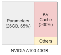
KV cache per token = 2 \(\times\)96\(\times\) (96 \(\times\) 128) \(\times\) 4
= 9.4 MB
For 2K context length = 2048 \(\times\) 9.4 MB
= 19.3 GB
to generate a sequence of length 2K requires 19.3 GB of memory for KV caching alone (we can't even use an A100 40 GB GPU).
A practical solution is to drop the keys and values of tokens that occured in the distant past (act similar to local windowed attention).
The other approach is to introduce model level modifications!
Multi-Query Attention (MQA)
KV cache per token (in B) =
2 \(\times\) num_layers \(\times\) (num_heads \(\times\) dim_head) \(\times\) precision_in_bytes
Select one hyper-parameter out of three hyperparameters that we could exploit in the formula to reduce the memory requirement is ____
Let's set \(num\_heads=1\) (it does not imply we use only one head). The number 2 in the formula means that we access two vectors (key-value) for each head.
Therefore, it means we want to access key-value pairs once for all the heads!
How can we do that?
Share all the key-value pairs across the heads.
Cache Memory
This greatly reduces the cache memory. However, the performance degrades significantly.
Moreover, this requires us to re-train the model with at least 5% of training data
k_1
k_2
k_3
v_1
v_2
v_3
Q_1
K-shared
V-shared
SM(Q_iK_i^T)V_i^T
Grouped-Query Attention (GQA)
On one extreme we have Multi-Head Attention where each head has a separate query, key and value vector.
On the other extreme we have Multi-Query Attention where each head has separate query but keys and values are shared across all heads.
Grouped Query Attention is just a middle ground between the two, where a group of queries share key-value pairs that result in performance close to MHA

Paged Attention (PA)
Typically, fixed and contiguous memory is reserved for KV-caching (say, based on context length of the model).
However, we do not know the length of the sequence that the model generates a priori.
The memory during the generation process is wasted if the model generated a sequence that is much smaller than the pre-fixed length.
A solution is to use a block of non-contiguous memory locations.
That is what Paged Attention does


References
Important Question
Can we sparsify Causal mask attention?
What happens during inference?
What happens for masked attention? Remember we add mask matrix to QK^T, so it does not matter (my guess)
Local attention and blockwise attention trades-off performance
Can we replace a transformer model trained with full attention by sparse attention during inference?
New attention layer: Lambda Layer
Various Ideas
New attention layer: Lambda Layer
Methods that embraces the limitation and a build a mechanism around it
Pre-trained Model with parametric memory (implicit knowledge)
World knowledge in non-parametric memory (explicit-knowledge)
Pre-trained Neural Retriever

2. Sliding Window
Second line of work questions if full attention is essential and have tried to come up with approaches that do not require full attention, thereby reducing the memory and computation requirements.
Unidirectional:
Bidirectional:
these approximations do not come with theoretical guarantees.
Random Attention: (From graph theory perspective)
- Random graph following Erdos-Rényi model
- the shortest path between any two nodes is logarithmic in the number of nodes with \(O(n)\) edges


Connected
Local attention

Random attention
The weight of an edge denotes the similarity score between nodes
its second eigenvalue (of the adjacency matrix) is quite far from the first eigenvalue
Global attention:
make some existing tokens “global”, which attend over the entire sequence
Two variants: ITC, ETC (extended tokens)
Question on Attention
What aspects of the self-attention model are necessary for its performance?
Can we achieve the empirical benefits of a fully quadratic self-attention scheme using fewer inner-products?
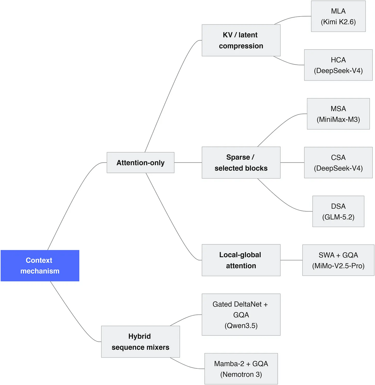
Attention used by open-frontier models - source
MAMBA: Linear time state space models
LongFormer
a drop-in replacement for the standard self-attention and combines a local windowed attention with a task motivated global attention.
scales linearly with the sequence length
can act as a drop-in replacement for the self-attention mechanism in pretrained Transformers (take existing check point, and Longformer attention during fine tuning)
BIGBIRD
We show that BIGBIRD is a universal approximator of sequence functions and is Turing complete, thereby preserving these properties of the quadratic, full attention model.
Visual inspection showed that most layers had sparse attention patterns across most data points, suggesting that some form of sparsity could be introduced without significantly affecting performance. [Ref]
Motivation for sparse attention
Brief Intro to GPU architecture

Compute: Arithmetic and other instructions are executed by the SMs (streaming multiprocessors)
Storage: data and code are accessed from DRAM (a.k.a, High Band width Memory (HBM)) via the L2 cache
| Model | num of SM | L2 cache | HBM (DRAM) | Band Width |
|---|---|---|---|---|
| A100 | 108 | 40MB | 80 GB | upto 2TB/s |
Streaming Multiprocessors

Each SM has its own instruction schedulers and various instruction execution pipelines

Core operation: Multiply and add
There are 512 TF32 cores in a single SM of A100.
Each core execute one Multiply and Add operation per clock
Therefore, FLOPs per clock is simply two times the number of cores. That is, 1024 FLOPs per clock
With 1.4 GHz clock frequency, this translates to 1.43 TFLOPS (Tera FLOPs per Second)
With 108 SM's, the overall peak throughput is 154 TF32 TFLOPS
Streaming Multiprocessors
At runtime, a thread block is placed on an SM for execution, enabling all threads in a thread block to communicate and synchronize efficiently
Launching a function with a single thread block would only give work to a single SM, therefore to fully utilize a GPU with multiple SMs one needs to launch many thread blocks
Since an SM can execute multiple thread blocks concurrently, typically one wants the number of thread blocks to be several times higher than the number of SMs

Launching a function with a single thread block would only give work to a single SM, therefore to fully utilize a GPU with multiple SMs one needs to launch many thread blocks. (The reason why people ignore batch of samples if number of samples is less than batch size)
How tensor cores differ from Cuda Cores?
Tensor cores accelerate matrix multiply and accumulate operations by operating on small matrix blocks (say, 4x4 blocks)
When math operations cannot be formulated in terms of matrix blocks they are executed in other CUDA cores
Performance Measure
- Math bandwidth
- Memory bandwidth
- latency
Task: Read ips - Do Math - Write ops
\(T_{mem}\): Time to read inputs from memory
\(T_{math}\): Time to perform the operation
Total time= \(max(T_{mem},T_{math}\))
If math time is longer we say that a function is math limited (bounded), if memory time is longer then it is memory limited (bounded).
T_{mem}>T_{math}
Suppose the algorithm is memory-bound
T_{mem}=\frac{\# bytes}{BW_{mem}}
T_{math}=\frac{\# OPs}{BW_{math}}
then we can write
\frac{\# bytes}{BW_{mem}}>
\frac{\# OPs}{BW_{math}}
\frac{BW_{math}}{BW_{mem}}>
\frac{\# OPs}{\#bytes}
arithmetic intensity
ops by bytes ratio
\frac{BW_{math}}{BW_{mem}}>
\frac{\# OPs}{\#bytes}
Multi-head attention is Memory bound
The arithmetic intensity is less than the OPs per Byte ratio
That is, the algorithm spend more time on reading and writing to memory than on the math operations (compute)!
How much time is spent in memory or math operations depends on both the algorithm and its implementation, as well as the processor’s bandwidths
Can we re-write the attention algorithm such that it spends less time in reading from and writing to memory? That is, can we translate all element wise operation in MHA to mat-mul ops? or use kernel fusion? Make it IO aware
To Do:
Display the algorithm for self-attention
Say we have two matrices of size 100 by 100 and want to do matrix multiplication
First we need to access all the 20000 elements, amounts to 80KB (4 byte per element)
Compute is: \(2 \times 100^3\)= 20 million
Artithmatic intensity = \(\frac{20 \times 10^6}{80 \times 10^3}=250\)
Ops-per-Byte = \(\frac{19 \times 10^{12} }{1 \times 10^{12}}=19\)
Say we have a matrix of size 100 by 100 and want to scale it by 2
First we need to access all the 10000 elements, amounts to 40KB (4 byte per element)
Compute is: \(10000\)= 10000
Artithmatic intensity = \(\frac{10000}{40000}=0.25\)
Ops-per-Byte = \(\frac{19 \times 10^{12} }{1 \times 10^{12}}=19\)

Lecture-8-Fast Attention Mechanisms
By Arun Prakash


