PCA-Kernel PCA
Arun Prakash A
Steps
X \in \mathbb{R}^{n \times d}

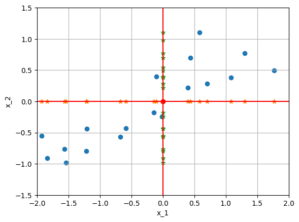
X \in \mathbb{R}^{20 \times 2}
Center the datapoints. Why?
\mu=\sum \limits_{i=1}^{n} x_i,\quad \mu \in\mathbb{R}^{1 \times d}
\(n\): # of samples, \(d\): # of features
X = X-\mu

Compute the covariance of ___?
(Different from lecture)
Compute the covariance of features
X=\begin{bmatrix}x_{11}&x_{12}\\
x_{21}&x_{22}
\end{bmatrix}
f_1
f_2
What is the sample variance for the features \(f_1,f_2\) (given that mean is zero)?
var(f_1)=\frac{1}{2}\sum x_{11}^2+x_{21}^2
for \(n\) samples,
var(f_1)=\frac{1}{n}\sum x_{11}^2+x_{21}^2+\cdots+x_{n1}^2
That is, simply square the elements of first column and sum them up
Repeat the same to compute the variance for all features
What is the sample co-variance between the features \(f_1,f_2\) (given that mean is zero)?
cov(f_1,f_2)=\frac{1}{2}\sum x_{11}x_{12}+x_{21}x_{22}
var(x)=\sum (x-\mu)^2p(x)
cov(x,y)=\sum (x-\mu_x)(y-\mu_y)p(x,y)
C=\frac{1}{n}X^TX
C=\frac{1}{n}X^TX
\begin{bmatrix}x_{11}&x_{12}\\
x_{21}&x_{22}
\end{bmatrix}
=\begin{bmatrix}x_{11}&x_{21}\\
x_{12}&x_{22}
\end{bmatrix}
=\begin{bmatrix}x_{11}^2+x_{21}^2 & x_{11}x_{12}+x_{21}x_{22}\\
x_{12}x_{11}+x_{22}x_{21} & x_{12}^2+x_{22}^2
\end{bmatrix}
Variance of feature 1
Variance of feature 2
=\begin{bmatrix}1.6& 0.7\\
0.7 &0.4
\end{bmatrix}
What does \(var(x)=1.6\) compared to \(var(x)=0.4\) , mean?
Roughly, the data spread along \(x-axis\) two times more than along \(y-axis\) (in the canonical bases)
What does \(var(x)=1.6\) compared to \(var(x)=0.4\) , mean?
Roughly, the datapoints spread along \(x-axis\) two times more than along \(y-axis\) (in the canonical bases)
=\begin{bmatrix}1.6& 0.7\\
0.7 &0.4
\end{bmatrix}
Moreover, the diagonal elements say that \(x\) and \(y\) are positively correlated.
We want to decorrelate the features and maximize the variance in a particular direction (say \(x\))
\begin{bmatrix}1.6\uparrow& 0\\
0 &0.4\downarrow
\end{bmatrix}
We look for other bases (direction)?
C = Q \Lambda Q^T
=\begin{bmatrix}0.9& -0.4\\
0.4 &0.9
\end{bmatrix}
\begin{bmatrix}1.99& 0\\
0 &0.08
\end{bmatrix}
\begin{bmatrix}0.9& 0.4\\
-0.4 &0.9
\end{bmatrix}

Rotate data points by \(Q\)

X_{rot}
C=X_{rot}^TX_{rot}=
\begin{bmatrix}1.99& 0\\
0 &0.08
\end{bmatrix}
Features are decorrelated!
Eigen vectors are the principal directions
The coordinate (eigenvalue) of the Eigen vectors are the principal components
Dual Formulation
X \in \mathbb{R}^{n \times d}
d>>n
X \in \mathbb{R}^{4 \times 10}
K=XX^T \in \mathbb{R}^{4 \times 4}
K=XX^T
K_{11}=x_{11}^2+x_{12}^2+\cdots+x_{10}^2
Is this a covariance matrix ?
No. Why?
K_{11}=x_{11}^2+x_{21}^2+\cdots+x_{10,1}^2
For it to be a variance
However, we have
Sum square of all the features in the first sample
Sum square of the first feature in all the samples
But \(K\) is a Symmteric Matrix!
nC=X^TX \in \mathbb{R}^{10 \times 10}
For example
Is there a relation ship between eigen vectors of \(K\) and \(C\)?
Is there a relation ship between eigenvalues of \(K\) and \(C\)?
Eigenvector of \(C\):
Cw_k=\lambda_kw_k
What is the size of the eigenvector?
X \in \mathbb{R}^{4 \times 10}
K=XX^T \in \mathbb{R}^{4 \times 4}
nC=X^TX \in \mathbb{R}^{10 \times 10}
w_k \in \mathbb{R}^{10}
Eigenvector of \(K\):
K\alpha_k=(n\lambda_k)\alpha_k
What is the size of the eigenvector?
a_k \in \mathbb{R}^{4}
We might need a transformation matrix that maps these eigenvectors!
w_k \in \mathbb{R}^{10}
a_k \in \mathbb{R}^{4}
Let's Jump in!
C=\frac{1}{n}X^TX
Cw_k=\lambda_kw_k
,Let \(w_k\) be the \(k-th\) eigen vector of \(C\)
\frac{1}{n\lambda_k}X^T(Xw_k)=w_k
\alpha_k=Xw_k
w_k= \frac{1}{n \lambda_k}(X^T\alpha_k)
w_k= \frac{1}{n \lambda}(\alpha_{k1}X^T[:,1]+\alpha_{k2}X^T[:,2]+\\\alpha_{k3}X^T[:,3]+\alpha_{k4}X^T[:,4])
\(w_k\) is a linear combination of all data points
Cw_k=\lambda_kw_k
w_k= \frac{1}{n \lambda_k}(X^T\alpha_k)
C\Big(\frac{1}{n \lambda_k}(X^T\alpha_k)\Big)=\lambda_k\Big(\frac{1}{n \lambda_k}(X^T\alpha_k)\Big)
X^TXX^T\alpha_k=n\lambda_kX^T\alpha_k
Multiply both sides by \(X\)
(XX^T)(XX^T)\alpha_k=n\lambda_k(XX^T)\alpha_k
(XX^T)\alpha_k=n\lambda_k\alpha_k
K\alpha_k=n\lambda_k\alpha_k
Therefore, \(\alpha_k\) is the eigen vector of \(K\)
How do we find the \(\alpha_k\)?
Substitute
in
K\alpha_k=n\lambda_k\alpha_k
Imposing unit norm condition: \(w_k^Tw_k\)=1
w_k= \frac{1}{n \lambda_k}(X^T\alpha_k)
\frac{1}{n^2 \lambda_k^2}(\alpha_k^TXX^T\alpha_k)=1
\frac{1}{n^2 \lambda_k^2}(\alpha_k^TK\alpha_k)=1
\frac{1}{n^2 \lambda_k^2}(\alpha_k^T n\lambda_k\alpha_k)=1
Replace \(K\alpha_k\) by
K\alpha_k=n\lambda_k\alpha_k
\frac{1}{n \lambda_k}(\alpha_k^T \alpha_k)=1
\frac{1}{n \lambda_k}(\sqrt{n \lambda_k}\alpha_k^T)(\sqrt{n \lambda_k} \alpha_k)=1
\beta_k=\sqrt{n \lambda_k}\alpha_k
\alpha_k=\frac{\beta_k}{\sqrt{n \lambda_k}}
Algorithm
Compute \(K=XX^T \in \mathbb{R}^{n \times n}\)
FInd the eigenvalues (\(n\lambda_1,n\lambda_2,\cdots,n\lambda_n\)) and eigenvectors (\(\alpha_1,\alpha_2,\cdots,\alpha_n\))
Scale down the eigenvectors (\(\alpha_1,\alpha_2,\cdots,\alpha_n\)) by square root of its eigenvalues.
Transform the scaled down eigenvectors by \(X^T\)
w_k =X^T \frac{\alpha_k}{\sqrt{n\lambda_k}}
\mathbb{R}^{d \times 1}
\mathbb{R}^{n \times 1}
\mathbb{R}^{d \times n}
C \rightarrow \lambda_1,\lambda_2,\cdots,\lambda_d
n>>d
d>>n
C \rightarrow \lambda_1,\lambda_2,\cdots,\lambda_n,\cdots,\lambda_d
K \rightarrow \lambda_1,\lambda_2,\cdots,\lambda_n
The eigenvalues are non-negative as \(C\) is positive semi-definite.
The eigenvalues are non-negative as \(K\) is a Gram-Matrix which is positive semi-definite.
X \in \mathbb{R}^{20 \times 2}
C \in \mathbb{R}^{2 \times 2}
C \rightarrow \lambda_1,\lambda_2
C \in \mathbb{R}^{10 \times 10}
X \in \mathbb{R}^{4 \times 10}
C \rightarrow \lambda_1,\lambda_2, \lambda_3,\lambda_4,\cdots \lambda_{10}
K \in \mathbb{R}^{4 \times 4}
K \rightarrow \lambda_1,\lambda_2,\lambda_3,\lambda_{4}
Important Observation
C
Each element in \(C\) is coming out of inner-product of elements from the set \(X\)
K
Each element in \(K\) is coming out of inner-product of elements from the set \(X\)
Albeit, in different ways
X^TX
XX^T
So both matrices are Gram Matrix!
We can move back and forth between these formulations using the set \(X\) !
w_k =X^T \frac{\alpha_k}{\sqrt{n\lambda_k}}
\alpha_k =X w_k ?
Non-Linear Relationships
Dot product
x
y
Assuming \(x,y\) are normalized
x^Ty=c
Gives angle
Scalar projection
||x||=\sqrt{x^Tx}
Length of a vector
||x-y||=\sqrt{(x-y)^T(x-y)}
x
x
y
||x-y||

C=\begin{bmatrix}0.5 & 0\\
0 & 0.5
\end{bmatrix}
X \in \mathbb{R}^{10 \times 2}
C =\frac{1}{10} X^TX
x_{11}^2+x_{21}^2+\cdots+x_{10,1}^2=x_1^Tx_1
Interpretation-1: Similarity
x_1^Tx_1=x_2^Tx_2=0.5
x_1^Tx_2=x_2x_1^T=0
Similar in \(\mathbb{R}^{10}\) ( equals 1 if the vector is normalized)
Zero similarity in \(\mathbb{R}^{10}\)
Any better similarity measure?
Motivation
[x_1^2,x_2^2,\sqrt{2}x_1x_2]


[u=x_1^2,v=x_2^2,w=\sqrt{2}x_1x_2]
Ok. Polynomial transformation separates these data points
Suppose we want to project these onto a place. Where should we project?
On to the \(uv\) plane?
Motivation
[u=x_1^2,v=x_2^2,w=\sqrt{2}x_1x_2]
On to \(uv\) plane?

(0,0,0)
(0,0,0)
Motivation
[u=x_1^2,v=x_2^2,w=\sqrt{2}x_1x_2]
Datapoints in inputspace \(X\)
Datapoints in Feature space \(\Phi(X)\)
Projection in the Feature space \(\Phi(X)^T(?)\)
Replace ? with the Equation of the plane
(0,0,0)
(0,0,0)


(0,0,0)


Source:BernhardNow your turn to make sense of these pictures
C=\begin{bmatrix}0.5 & 0\\
0 & 0.5
\end{bmatrix}
Each element in the covariance matrix is a dot product between a row of \(X\) and a column of \(X^T\).
\mathbb{R}^2
f_1
f_2
(0,0)
(f_1-a)^2+(f_2-b)^2=r^2
Relation
[f_1,f_2] \in \mathbb{R}^2
\Phi(x_i)^Tu=0
What does this dot product say?
(a,b)
f_1^2+a^2-2f_1a+f_2^2+b^2-2f_2b-r^2=0
[f_1,f_2] \rightarrow
\begin{bmatrix}
1 & f_1^2 & f_2^2 & f_1f_2 & f_1 & f_2
\end{bmatrix}
u= \begin{bmatrix}
a^2+b^2-r^2 &1 & 1 & 0 &-2a & -2b
\end{bmatrix}
\Phi
Note the vector \(u\) is fixed given \(a,b,r\)
We transform each data point using \(\Phi\).
Then,
\Phi(x_i)^T
What does this dot product say?
\Phi
u=0
R^2
u
R^3?
Note the vector \(u\) is fixed.
Possible directions of \(\Phi\)?
\Phi

All the transformed datapoints now lie on a linear sub-space spanned by two independent vectors!
Note, however, that we do not know the distribution of the points in the transformed space. We only know that it is sitting in the linear subspace.
Objective: Find the principal components in the transformed subspace
C_{\Phi}=\frac{1}{n}\Phi(X^T)\Phi(X)
X \in \mathbb{R}^{n \times d}
X_{\Phi} \in \mathbb{R}^{n \times D}
D>>d
n
d
D
num of samples
num of features in \(\mathcal{X}\)
num of features in \(\mathbb{H}\)
n>>d
use \(C=X^TX\)
d>>n
use \(K=XX^T\)
D>>d
D>>n
Given that feature space could easily reach \(10^{10}\) dimension (or infinite)

32 \times 32
p=4
\(p\)-th order polynomial
^{1028}C_{4}=4.5^{10}
requires \(d^2\) dot products
requires \(n^2\) dot products
\(C_{\Phi}=\Phi(X)^T \Phi(X)\)
requires \(D^2\) dot products
\(K_{\Phi}=\Phi(X) \Phi(X)^T\)
requires \(n^2\) dot products
Computing \(\Phi(x)\) in itself is infeasible!
\mathcal{X}
\mathbb{H}
Lower dimensional input space
Higher (including infinite) dimensional Feature space (aka,Hilbert Space)
The computation in \(\mathcal{X}\) that induces inner prodcut in \(\mathbb{H}\)
\Phi(\cdot)
In practice, dim of \(10^{10},10^{15}\) could easily occur
A Kernel function does that
k:\mathcal{X} \times \mathcal{X} \rightarrow \mathbb{R}
\forall x,x'\in\mathcal{X}, k(x,x')=
Carrying out inner product is costly. Say, we need \(10^{10}\) multiplications and additions to compute single dot product
\Phi(x)^T\Phi(x')
Polynomial Kernel
\forall x,x'\in\mathcal{X}, k(x,x')=
\Phi(x)^T\Phi(x')
(x_i^Tx_j+1)^2
x=\begin{bmatrix}
f_1&f_2
\end{bmatrix}
x'=\begin{bmatrix}
g_1&g_2
\end{bmatrix}
x^Tx'=\begin{bmatrix}
f_1g_1+f_2g_2
\end{bmatrix}
(x^Tx'+1)^2=(
f_1g_1+f_2g_2+1)^2
\Phi(x)^T\Phi(x')
\Phi(x)^T=\begin{bmatrix}f_1^2 &f_2^2 & 1 &\sqrt{2}f_1f_2 & \sqrt{1} & \sqrt{2}
\end{bmatrix}
Is equal to transforming the data point by
and computing the inner product
Therefore, the \(ij-th\) element of covariance matrix in the feature space is given by \(ij-th\) element of \(K\):
K_{ij}=
k:(x_i^Tx_j+1)^{2}
Computational complexity: Polynomial transformation of degree 10
X \in \mathbb{R}^{100 \times 6}
X_\Phi \in \mathbb{R}^{100 \times 8008}
C \in \mathbb{R}^{6\times6}
C_\Phi \in \mathbb{R}^{8008\times8008}
[We do not directly compute this]
k:(x_i^Tx_j+1)^{10}
C_\Phi=\begin{bmatrix}
\Phi(x_1)^T\Phi(x_1) & \Phi(x_1)^T\Phi(x_2) &\cdots&\Phi(x_1)^T\Phi(x_{8008}) \\
\vdots & \vdots & \ddots &\vdots
\end{bmatrix}
We are now facing a problem.
How do we compute
\Phi(x_1)^T\Phi(x_7)?=(x_1^Tx_7+1)^{10}
We do not have \(x_7\)? or any of \(x_i, i>6\).
What could be the solution?
Computational complexity: Polynomial transformation of degree 10
X \in \mathbb{R}^{100 \times 6}
X_\Phi \in \mathbb{R}^{100 \times 8008}
K \in \mathbb{R}^{100\times100}
K_\Phi \in \mathbb{R}^{100\times100}
[We do not directly compute this]
k:(x_i^Tx_j+1)^{10}
K_\Phi=\begin{bmatrix}
\Phi(x_1)^T\Phi(x_1) & \Phi(x_1)^T\Phi(x_2) &\cdots&\Phi(x_1)^T\Phi(x_{100}) \\
\vdots & \vdots & \ddots &\vdots
\end{bmatrix}
Interesting part is here,
We have already computed this in \(K\)
Use this:
(K+\mathbf{1})^{10}
(K+\mathbf{1})^{10}
We already know how to move from \(K\) to \(C\)
Computational complexity: Polynomial transformation of degree 10
X_\Phi \in \mathbb{R}^{100 \times 8008}
K_\Phi \in \mathbb{R}^{100\times100}
[We do not directly compute this]
K_\Phi=\begin{bmatrix}
\Phi(x_1)^T\Phi(x_1) & \Phi(x_1)^T\Phi(x_2) &\cdots&\Phi(x_1)^T\Phi(x_{100}) \\
\vdots & \vdots & \ddots &\vdots
\end{bmatrix}
(K+\mathbf{1})^{10}
The dataset \(X_\Phi\) is not centered.
We can center it by computing mean of \(X_\Phi\). However, we can not, because...?
Therefore, center the Kernel
Compute eigenvector \(w_k^\Phi\) using
w_k^\Phi=X_\Phi\frac{\alpha_k^\Phi}{\sqrt{n\lambda_k^\Phi}}
Once again we never compute \(X_\Phi\)
Why do we need eigenvectors if all that we need is compression?
\Phi(x_i)^Tw_k^\Phi \rightarrow
Projection of the transformed point on to the k-th eigenvector of \(K_\Phi\)
\Phi(x_i)^Tw_k^\Phi =
\Phi(x_i)^T\sum \limits_{j=1}^n \Phi(x_j)\alpha_{kj}^\Phi
=\sum \limits_{j=1}^n \Phi(x_i)^T\Phi(x_j)\alpha_{kj}^\Phi
=\sum \limits_{j=1}^n K_{ij}^{\Phi}\alpha_{kj}^\Phi
\mathbf K^C = \mathbf K - \mathbf 1_n \mathbf K - \mathbf K \mathbf 1_n + \mathbf 1_n \mathbf K \mathbf 1_n
\mathbf 1_n=\frac{1}{n}\begin{bmatrix}&np.ones(&\\
&n \times n)&\\
\end{bmatrix}
Can any function
\mathsf{K}(\cdot,\cdot)\rightarrow{\mathbb{R}}
be a kernel?
The transformation has to be a real inner product
x \rightarrow\Phi(x)
y \rightarrow\Phi(y)
\mathsf{k}(x,y) \rightarrow \langle \Phi(x),\Phi(y) \rangle
\Phi(\cdot) \rightarrow
\Phi(\cdot) \rightarrow
Linear
Guassian/radial
\Phi(\cdot) \rightarrow
Exponential, laplacian
\Phi(\cdot) \rightarrow
sigmoidal
\Phi(\cdot) \rightarrow
All Polynomial transformation
K(x,y)=x^Ty
K(x,y)=(1+x^Ty)^d
K(x,y)=exp(\frac{-||x-y||^2}{\sigma^2})
K(x,y)=exp(\frac{-||x-y||^2}{2\sigma^2})
K(x,y)=exp(\frac{-||x-y||}{\sigma})
K(x,y)=tanh(x^Ty+c)
Summary
X \in \mathbb{R}^{n \times d}
\mu=\sum \limits_{i=1}^{n} x_i,\quad \mu \in\mathbb{R}^{1 \times d}
X = X-\mu
C=\frac{1}{n}X^TX
C=Q\Lambda Q^T
(\lambda_k,w_k)
kth eigen-value and eigenvector is
Summary
X \in \mathbb{R}^{n \times d}
\mu=\sum \limits_{i=1}^{n} x_i,\quad \mu \in\mathbb{R}^{1 \times d}
X = X-\mu
C=\frac{1}{n}X^TX
C=Q\Lambda Q^T
(\lambda_k,\mathbf{w_k})
kth eigen-value and eigenvector is
K=XX^T
(n\lambda_k,\mathbf{\alpha_k})
Transform the scaled down eigenvectors by \(X^T\)
w_k =X^T \frac{\alpha_k}{\sqrt{n\lambda_k}}
\mathbb{R}^{d \times 1}
\mathbb{R}^{n \times 1}
\mathbb{R}^{d \times n}
d>>n
n
d
D
num of samples
num of features in \(\mathcal{X}\)
num of features in \(\mathbb{H}\)
n>>d
use \(C=X^TX\)
d>>n
use \(K=XX^T\)
D>>d
D>>n
Given that feature space could easily reach \(10^{10}\) dimension (or infinite)
32 \times 32
p=4
\(p\)-th order polynomial
^{1028}C_{4}=4.5^{10}
requires \(d^2\) dot products
requires \(n^2\) dot products
\(C_{\Phi}=\Phi(X)^T \Phi(X)\)
requires \(D^2\) dot products
\(K_{\Phi}=\Phi(X) \Phi(X)^T\)
requires \(n^2\) dot products
Computing \(\Phi(x)\) in itself is infeasible!
Computational complexity: Polynomial transformation of degree 10
X \in \mathbb{R}^{100 \times 6}
X_\Phi \in \mathbb{R}^{100 \times 8008}
K \in \mathbb{R}^{100\times100}
K_\Phi \in \mathbb{R}^{100\times100}
[We do not directly compute this]
k:(x_i^Tx_j+1)^{10}
K_\Phi=\begin{bmatrix}
\Phi(x_1)^T\Phi(x_1) & \Phi(x_1)^T\Phi(x_2) &\cdots&\Phi(x_1)^T\Phi(x_{100}) \\
\vdots & \vdots & \ddots &\vdots
\end{bmatrix}
Interesting part is here,
We have already computed this in \(K\)
Use this:
(K+\mathbf{1})^{10}
(K+\mathbf{1})^{10}
We already know how to move from \(K\) to \(C\)
Computational complexity: Polynomial transformation of degree 10
X_\Phi \in \mathbb{R}^{100 \times 8008}
K_\Phi \in \mathbb{R}^{100\times100}
[We do not directly compute this]
K_\Phi=\begin{bmatrix}
\Phi(x_1)^T\Phi(x_1) & \Phi(x_1)^T\Phi(x_2) &\cdots&\Phi(x_1)^T\Phi(x_{100}) \\
\vdots & \vdots & \ddots &\vdots
\end{bmatrix}
(K+\mathbf{1})^{10}
The dataset \(X_\Phi\) is not centered.
We can center it by computing mean of \(X_\Phi\). However, we can not, because...?
Therefore, center the Kernel
Compute eigenvector \(w_k^\Phi\) using
w_k^\Phi=X_\Phi\frac{\alpha_k^\Phi}{\sqrt{n\lambda_k^\Phi}}
Once again we never compute \(X_\Phi\)
\Phi(x_i)^Tw_k^\Phi =
\Phi(x_i)^T\sum \limits_{j=1}^n \Phi(x_j)\alpha_{kj}^\Phi
=\sum \limits_{j=1}^n \Phi(x_i)^T\Phi(x_j)\alpha_{kj}^\Phi
=\sum \limits_{j=1}^n K_{ij}^{\Phi}\alpha_{kj}^\Phi
Why do we need eigenvectors if all that we need is compression?
Kernel-PCA-MLT
By Arun Prakash
Kernel-PCA-MLT
A presentation used in Machine Learning Techniques Week-2 live session


