
Developing Deep Learning Models using
Arun Prakash A
IIT Madras
Core: tensors
JIT
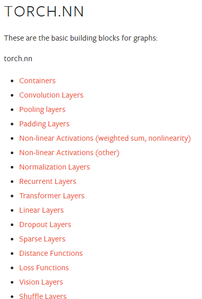
nn
Optim
multiprocessing
quantization
sparse
ONNX
Distributed
fast.ai
Detectron 2
Horovod
Flair
AllenNLP
torch.vision
BoTorch
GloW
Lightening
Skorch

import torch
import torch.nn as nn
import torch.nn.functional as F

class Model(nn.Module):

    def __init__(self, num_hidden):
        super(Model, self).__init__()
        self.layer1 = nn.Linear(28 * 28, 100)
        self.layer2 = nn.Linear(100, 50)
        self.layer3 = nn.Linear(50, 20)
        self.layer4 = nn.Linear(20, 1)
        self.num_hidden = num_hidden
    def forward(self, img):
        flattened = img.view(-1, 28 * 28)
        activation1 = F.relu(self.layer1(flattened))
        activation2 = F.relu(self.layer2(activation1))
        activation3 = F.relu(self.layer3(activation2))
        output = self.layer4(activation3)
        return output
The objective is not only
Build-Train-Test Deep Learning models
but also to Debug
Debugging requires a deeper understanding of things happening under the hood!
For the next two sessions, you most likely feel you are not doing deep learning
The Software Architecture of PyTorch
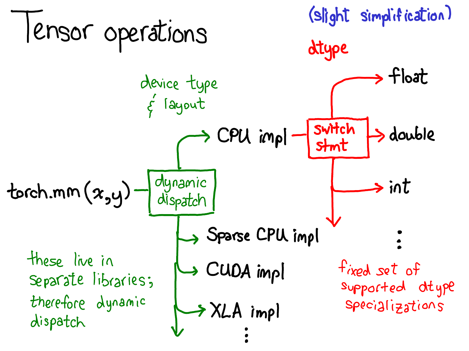
Tensor in
Tensor out
Operations on Tensors
Parameter Tensor in

Framework


What I build
Industry
Tech Giants
JIT
Cpp
Autograd
Cpp
TH
THC
Python
API
"A Tensor": ATen
"Caffe2 10": C10
Hardware Specific
torch
torch.autograd
torch.nn
torch. utils
CUDA,CPU,AMD,METAL
Tensor computation (like NumPy) with strong GPU acceleration
Deep neural networks built on a tape-based autograd system
Support efficient industry production at massive scale
Support exporting models to Python-less environment
Support for platforms of Caffe2 (iOS, Android, Raspbian, Tegra, etc) and will continue to expand various platforms support
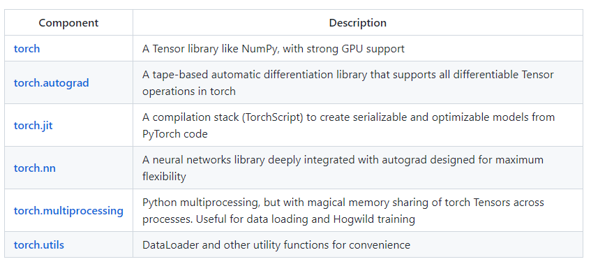
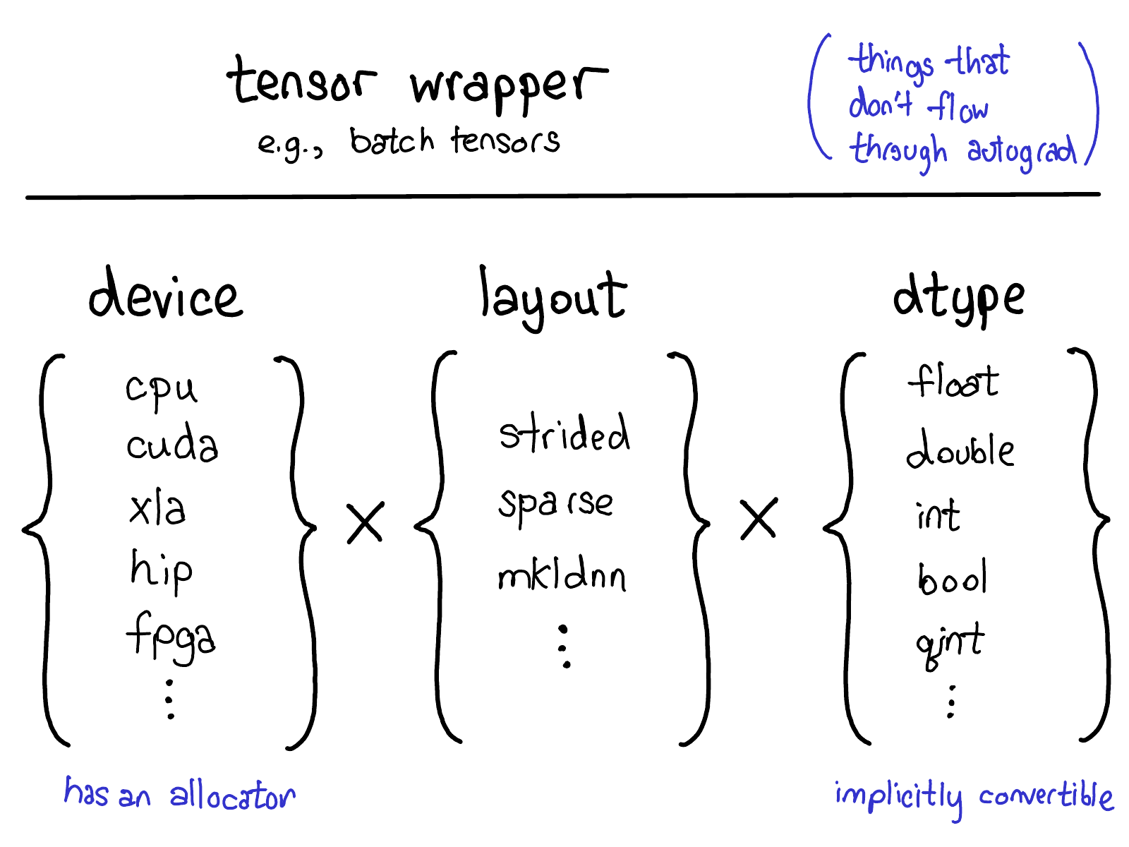
torch.utils.data (now, TorchData)TorchVision, TorchText modulestorch.tensor()

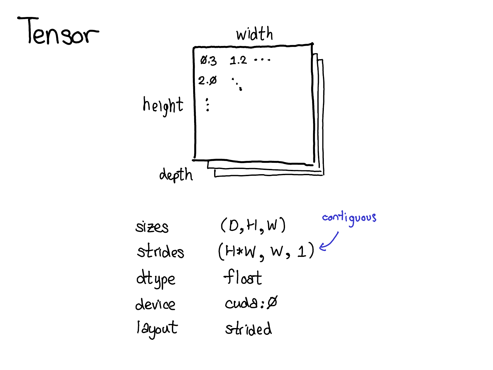
tensors
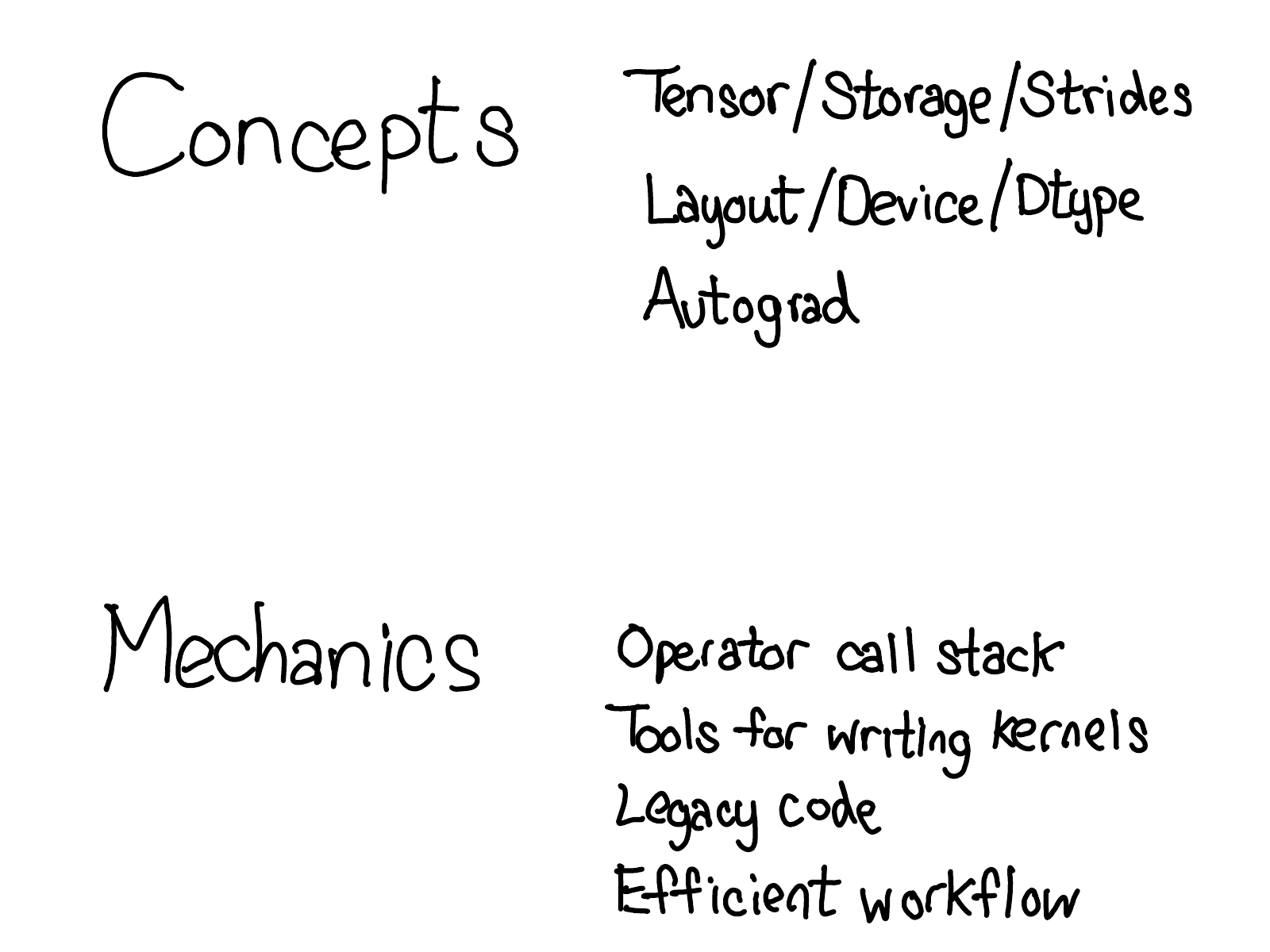
Concepts
Logical (view)

Physical
(Storage)
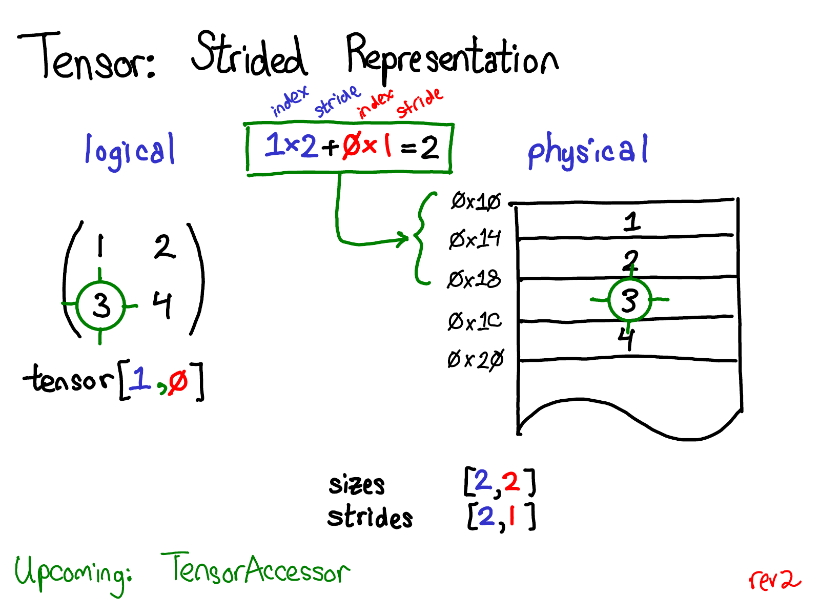
Stride
(Indexing)
Memory Layout

Devices

| 1 | 1.0 | 2 | 2.0 |
|---|
dtype
Limitations of using pure Python
List in python is in fact Linked List (Dynamic Array) under the hood
Python GIL (Global Interpreter Lock) which prevents Multiprocessing
This in turn affects the model training time (inevitably)
Why should I Learn the internals?
Suppose we have a matrix of size \(X = 1000 \times 1000\)
Is transposing a costly operation?
How do you write a code to transpose? Looping?
Does accessing elements take constant time?
We can answer questions like these if we know how the tensors are actually stored in a hardware.
Is computing len(x) a costly operation?
| Tensor |
|---|
| storage |
| stride |
| shape |
| device |
| size |
| grad |
| grad_fn |
| ndim |
Tensor Object
\lbrace
Some useful/important attributes of a pytorch tensor
x
x = torch. Tensor([])| Tensor |
|---|
| storage |
| stride |
| shape |
| device |
| size |
| grad |
| grad_fn |
| ndim |
Tensor Object
Usually, all tensors are created in CPU (unless, explicitly set to GPU).
We can move back and forth between CPU and GPU, however, it is a costlier operation for a large tensors!
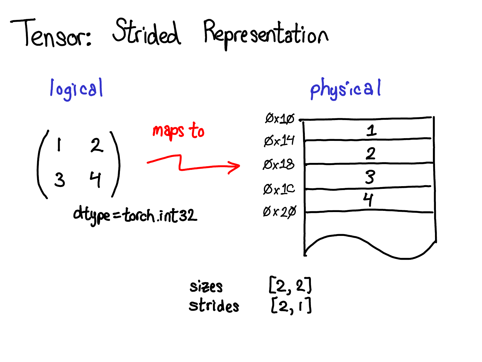
Maping follows a row-major form
The other representation is sparse representation
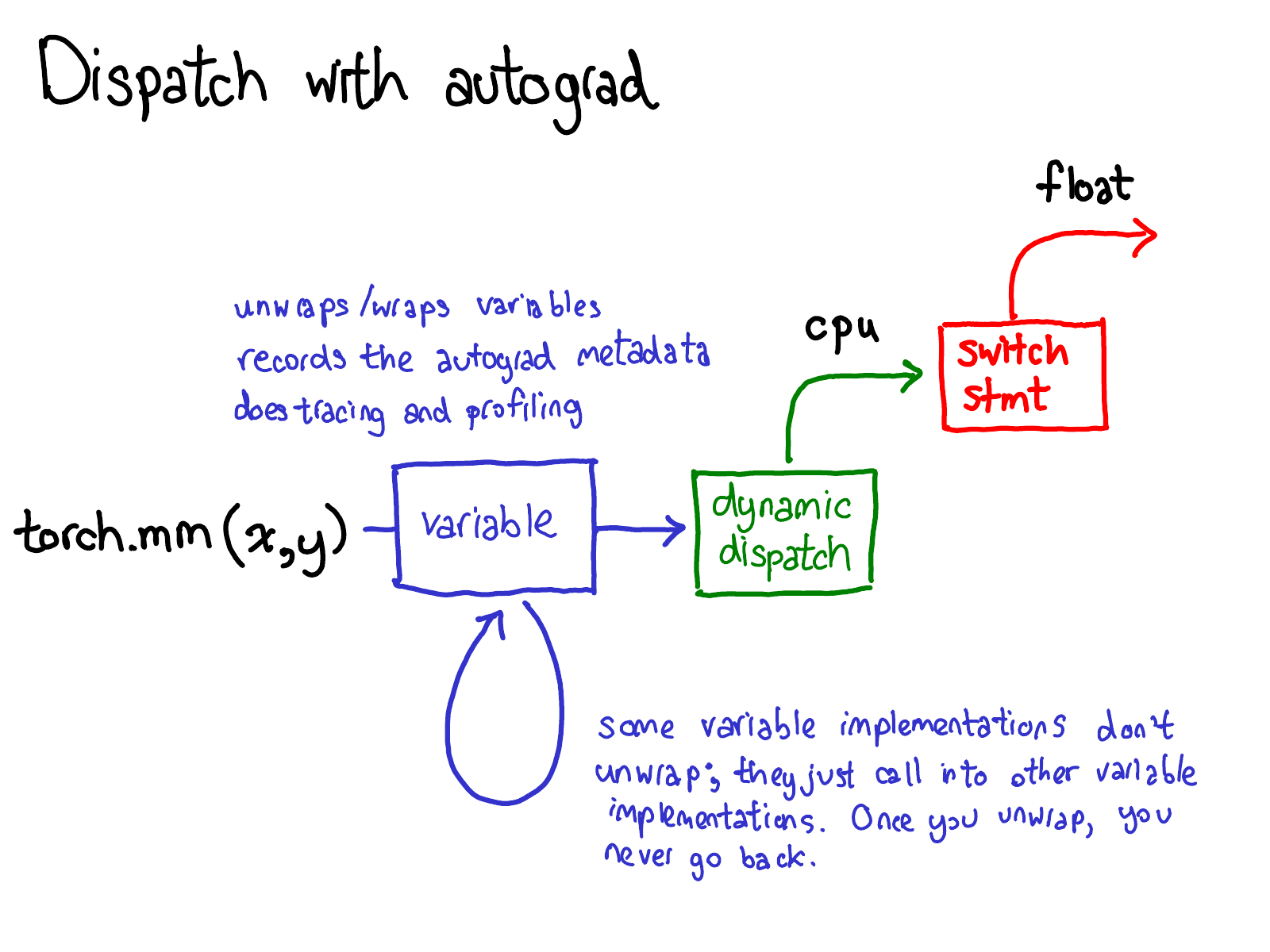
Dispatching


Physical storage
Logical View
Source:istock
Source:istock
Dimensions/axis/coordinate
| 0.1 |
|---|
x = torch. Tensor(0.1)x[0]invalid index of a 0-dim tensor
x.item()Dim: 0
Memory location
Dimensions/axis/coordinate
| 0.1 | 0.2 | 0.3 |
|---|
x = torch. Tensor([0.1,0.2,0.3])x[0]
>>0.1Dim: 1
Stride: 1
Contiguous memory
Dimensions/axis/coordinate
| 0.1 | 0.2 | 0.3 | 0.4 | 0.5 | 0.6 | 0.7 | 0.8 | 0.9 | 1 |
|---|
x = torch. Tensor([[0.1,0.2,0.3],[0.4,0.5,0.6],[0.7,0.8,0.9]])x[1]Dim: 2
stride: (3,1)
[d0*d0_stride + d1*d1_stride]
[1*3+
0*1 = 3]
It is alright to view this as a matrix but not always helpful when we deal with high dim tensors
Dimensions/axis/coordinate
| 0.1 | 0.2 | 0.3 | 0.4 | 0.5 | 0.6 | 0.7 | 0.8 | 0.9 | 1 |
|---|
x = torch. Tensor([[0.1,0.2,0.3],[0.4,0.5,0.6],[0.7,0.8,0.9]])torch.sum(x,dim=0)Dim: 2
stride: (3,1)
[d0*d0_stride + d1*d1_stride]
| 1.2 |
|---|
shape: (3,3)
Range:d0={0,1,2}
Range:d1={0,1,2}
since sum is across dim:0, vary dim:0 to its range (inner loop) and then dim:1 (outer loop)
0*3+ 0*1=0, x[0]=0.1
1*3+ 0*1=3, x[3]=0.4
2*3+ 0*1=6, x[6]=0.7
\sum
=1.2
Dimensions/axis/coordinate
| 0.1 | 0.2 | 0.3 | 0.4 | 0.5 | 0.6 | 0.7 | 0.8 | 0.9 | 1 |
|---|
x = torch. Tensor([[0.1,0.2,0.3],[0.4,0.5,0.6],[0.7,0.8,0.9]])torch.sum(x,dim=0)Dim: 2
stride: (3,1)
[d0*d0_stride + d1*d1_stride]
| 1.2 | 1.5 |
|---|
shape: (3,3)
Range:d0={0,1,2}
Range:d1={0,1,2}
since sum is across dim:0, vary dim:0 to its range (inner loop) and then dim:1 (outer loop)
0*3+ 1*1=1, x[1]=0.2
1*3+ 1*1=4, x[4]=0.5
2*3+ 1*1=7, x[7]=0.8
\sum
=1.5
Dimensions/axis/coordinate
| 0.1 | 0.2 | 0.3 | 0.4 | 0.5 | 0.6 | 0.7 | 0.8 | 0.9 | 1 |
|---|
x = torch. Tensor([[0.1,0.2,0.3],[0.4,0.5,0.6],[0.7,0.8,0.9]])torch.sum(x,dim=0)Dim: 2
stride: (3,1)
[d0*d0_stride + d1*d1_stride]
| 1.2 | 1.5 | 1.8 |
|---|
shape: (3,3)
Range:d0={0,1,2}
Range:d1={0,1,2}
since sum is across dim:0, vary dim:0 to its range (inner loop) and then dim:1 (outer loop)
0*3+ 2*1=2, x[1]=0.3
1*3+ 2*1=5, x[4]=0.6
2*3+ 2*1=8, x[7]=0.9
\sum
=1.8
Dimensions/axis/coordinate
| 0.1 | 0.2 | 0.3 | 0.4 | 0.5 | 0.6 | 0.7 | 0.8 | 0.9 | 1 |
|---|
x = torch. Tensor([[0.1,0.2,0.3],[0.4,0.5,0.6],[0.7,0.8,0.9]])torch.sum(x,dim=1)Dim: 2
stride: (3,1)
[d0*d0_stride + d1*d1_stride]
| 0.6 |
|---|
shape: (3,3)
Range:d0={0,1,2}
Range:d1={0,1,2}
since sum is across dim:1 now, vary dim:1 to its range (inner loop) and then dim:1 (outer loop)
0*3+ 0*1=0, x[0]=0.1
0*3+ 1*1=1, x[1]=0.2
0*3+ 2*1=2, x[2]=0.3
\sum
=0.6
Dimensions/axis/coordinate
| 0.1 | 0.2 | 0.3 | 0.4 | 0.5 | 0.6 | 0.7 | 0.8 | 0.9 | 1 |
|---|
x = torch. Tensor([[0.1,0.2,0.3],[0.4,0.5,0.6],[0.7,0.8,0.9]])torch.sum(x,dim=1)Dim: 2
stride: (3,1)
[d0*d0_stride + d1*d1_stride]
| 0.6 | 1.5 |
|---|
shape: (3,3)
Range:d0={0,1,2}
Range:d1={0,1,2}
since sum is across dim:1 now, vary dim:1 to its range (inner loop) and then dim:1 (outer loop)
1*3+ 0*1=3, x[3]=0.4
1*3+ 1*1=1, x[4]=0.5
1*3+ 2*1=2, x[5]=0.6
\sum
=1.5
Dimensions/axis/coordinate
| 0.1 | 0.2 | 0.3 | 0.4 | 0.5 | 0.6 | 0.7 | 0.8 |
|---|
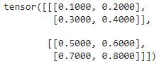
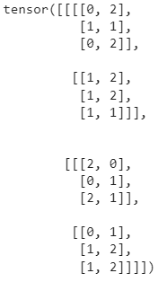
x = torch.tensor([[[0.1,0.2],[0.3,0.4]],[[0.5,0.6],[0.7,0.8]]])Dim: 3
torch.sum(x,dim=1)Let's figure out the shape of the tensor by starting with the right most dimension
\(d_k=2 \) (because there are two numbers (scalars) enclosed by a square bracket
\(d_{k-1} =2 \) (because there are two vectors (dim:1) enclosed by a square bracket
\(d_{k-2} =1 \)
Dimensions/axis/coordinate
| 0.1 | 0.2 | 0.3 | 0.4 | 0.5 | 0.6 | 0.7 | 0.8 |
|---|
x = torch.tensor([[[0.1,0.2],[0.3,0.4]],[[0.5,0.6],[0.7,0.8]]])Dim: 3
torch.sum(x,dim=1)stride: (4,2,1)
[d0*d0_stride + d1*d1_stride+d2*d2_stride]
shape: (1,2,2)
Range:d0={0,1,2}
Range:d1={0,1,2}
x:2 \times 2 \times 3 \times 2
torch.sum(x,dim=2)stride: (12,6,2,1)
Range:d0={0,1}
Range:d1={0,1}
Range:d2={0,1,2}
Range:d3={0,1}
| d0*12 | d1*6 | d2*2 | d3*1 |
|---|---|---|---|
| 0 | 0 | 0 | 0 |
| 1 | |||
| 2 |
index: 0+0+0+0=0, x[0]=0
index: 0+0+2+0=0, x[2]=1
index: 0+0+4+0=0, x[4]=0
\sum
=1
x:2 \times 2 \times 3 \times 2
torch.sum(x,dim=2)stride: (12,6,2,1)
Range:d0={0,1}
Range:d1={0,1}
Range:d2={0,1,2}
Range:d3={0,1}
| d0*12 | d1*6 | d2*2 | d3*1 |
|---|---|---|---|
| 0 | 0 | 0 | |
| 1 | 1 | ||
| 2 |
index: 0+0+0+1=1, x[1]=2
index: 0+0+2+1=3, x[3]=1
index: 0+0+4+1=0, x[5]=2
\sum
=5
Move into the right adjacent dimension
x:2 \times 2 \times 3 \times 2
torch.sum(x,dim=2)stride: (12,6,2,1)
Range:d0={0,1}
Range:d1={0,1}
Range:d2={0,1,2}
Range:d3={0,1}
| d0*12 | d1*6 | d2*2 | d3*1 |
|---|---|---|---|
| 0 | 0 | 0 | |
| 1 | 1 | ||
| 2 |
index: 0+6+0+0=6, x[6]=1
index: 0+6+2+0=8, x[8]=1
index: 0+6+4+0=10, x[10]=1
\sum
=3
Move into left adjacent dimension
x:2 \times 2 \times 3 \times 2
2 \times 2 \times 3 \times 2
We call the 'sum' a reduction operation as it reduces the dim from 3 to 1.
2 \times 2 \times 2
2 \times 3 \times 2
torch.sum(x,dim=2)torch.sum(x,dim=1)
2 \times 2 \times 3
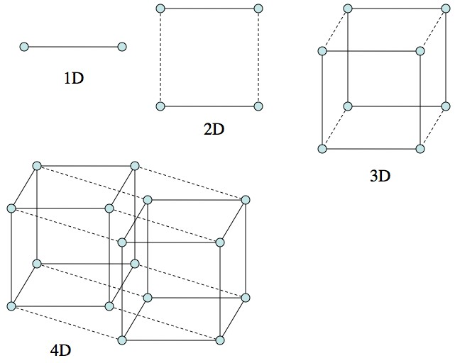
torch.sum(x,dim=3)3 \times 5 \times 5 \times 5
All these cubes are the elements at 0-th dim of a tensor of shape \(3 \times 5 \times 5 \times 5\). The first number 3 denotes three elements in zeroth dim and each of size 5 x 5 x 5 and
Let's switch to Colab Notebook
Cautions
1. Casting a Numpy array to a torch tensor ( vice-versa) shares a common memory (buffer). Changing one affects the other
2. Avoid in place operations (or be conscious of it) as it affects back prop and hence gives raise to unexpected results
torch.autograd()
Developing Deep Learning Models using
Pytorch
Arun Prakash A
DL Course Instructor
BS, IIT Madras
Recap
Tensor in
Tensor out
Operations on Tensors
Parameter Tensor in
Focus of the session!
| Tensor |
|---|
| storage |
| stride |
| shape |
| device |
| size |
| grad |
| grad_fn |
| req_grad |
| backward |
Tensor Object
Objective
Understnad how gradients are computed for a given tensor using a computational graph
\nabla w=\sum \quad(\hat{y}-y) \quad \sigma(x)(1-\sigma(x))\quad x
.grad_fn
(lossBackward)
.grad_fn
<sigmoidBackward>
ctx._savedTensor
Accumulate
.grad
Gradient computation for a single sigmoid neuron
Requirements to compute backprop for any NN?
| Forward Prop | Back-Prop |
|---|---|
|
|
|
|
|
|
|
|
|
|
|
(10+) Activation functions
Gradient function for those activation functions
Matmul, \(Wx\)
Gradient function for Matmul, \(W^T\)
Conv, \(W * x\)
Gradient function for convolution
In general, we need gradient functions for all the operations used in the forward propagation
ConCat, \([x_1, x_2]\)
Gradient function for concatenation
AutoGrad is not FiniteDiff
AutoGrad is tape-based autodiff
Maintain a list of functions (operators) with the way to compute gradients for them
def sigmoid():

  def propagate():

    pass
def tanh():

  def propagate():

    pass
def add():

  def propagate():

    pass
def matmul():

  def propagate():

    pass
z = x * y
x
*
y
z
def mul(x,y):
  z = x*y
\frac{\partial z}{\partial x}=y
*
\frac{\partial z}{\partial y}=x
\frac{\partial L}{ \partial z}
\frac{\partial L}{\partial x}=\frac{\partial L}{\partial z} \frac{\partial z}{\partial x}
\frac{\partial L}{\partial y}=\frac{\partial L}{\partial z} \frac{\partial z}{\partial y}
def mul(x,y):
  '''
  The clousre:
     Outer scope variables are x,y,z.
     These are binded to the nested function propagate for backprop
  '''
  z = x*y
  def propagate(dLdz):
    dLdx = dLdz*y
    dLdy = dLdz*x
    return (dLdx,dLdy)
    # store it in a tape
    gradient_tape.append([x,y,propagate])

  return z
\frac{\partial L}{\partial x}=\frac{\partial L}{\partial z} y
\frac{\partial L}{\partial y}=\frac{\partial L}{\partial z} x
grad_fn = <MulBackward>
z = x + y
x
+
y
z
\frac{\partial z}{\partial x}
+
\frac{\partial z}{\partial y}
\frac{\partial L}{ \partial z}
\frac{\partial L}{\partial x}=\frac{\partial L}{\partial z} \frac{\partial z}{\partial x}
\frac{\partial L}{\partial y}=\frac{\partial L}{\partial z} \frac{\partial z}{\partial y}
def add(x,y):
  '''
  The clousre:
     Outer scope variables are x,y,z.
     These are binded to the nested function propagate for backprop
  '''
  z = x+y
  def propagate(dLdz):
    dLdx = dLdz
    dLdy = dLdz
    return (dLdx,dLdy)
    # store it in a tape
    gradient_tape.append([x,y,propagate])

  return z
\frac{\partial L}{\partial x}=\frac{\partial L}{\partial z}
\frac{\partial L}{\partial y}=\frac{\partial L}{\partial z}
grad_fn = <AddBackward>
z = Wx+b
\frac{\partial z}{\partial x}
+
\frac{\partial L}{ \partial z}
\frac{\partial L}{\partial x}=\frac{\partial L}{\partial z} \frac{\partial z}{\partial x}
def matmul(x,y):
  '''
  The clousre:
     Outer scope variables are x,y,z.
     These are binded to the nested function propagate for backprop
  '''
  z = x+y
  def propagate(dLdz):
    dLdx = dLdz
    dLdy = dLdz
    return (dLdx,dLdy)
    # store it in a tape
    gradient_tape.append([x,y,propagate])

  return z
\frac{\partial L}{\partial x}= W^T\frac{\partial L}{\partial z}
grad_fn = <AddmmBackward>
Assuming denominator layout
z = \sigma(x)
\frac{\partial z}{\partial x}
\frac{\partial L}{ \partial z}
\frac{\partial L}{\partial x}=\frac{\partial L}{\partial z} \frac{\partial z}{\partial x}
def tanh(x):
  '''
  The clousre:
     Outer scope variables are x,y,z.
     These are binded to the nested function propagate for backprop
  '''
  z = sigmoid(x)

  def propagate(dLdz):
    dLdx = dLdz*dtanh(x)

    return (dLdx)
    # store it in a tape
    gradient_tape.append([x,propagate])

  return z
\frac{\partial L}{\partial x}=\frac{\partial L}{\partial z} \sigma'(x)
\sigma()
grad_fn = <TanhBackward>
Pytorch already has implemented forward-backward calls for so many Functions (Operations)
Those includes matmul, activation, add, slice,concat,..Let's call these as elementary functions for convenience
What if I want to implement the same for a new Function(operation)? (of course, it is less likely unless you are doing a research in the core domain)
from torch.autograd import Function

class FFT(Function):
     @staticmethod
     def forward(ctx, i,nfft):
        result = fft(i,nfft)
        ctx.save_for_backward(result)
        return result

     @staticmethod
     def backward(ctx, grad_output):
         result, = ctx.saved_tensors
        return grad_output * result

 # Use it by calling the apply method:
 output = FFT.apply(input)
from torch.autograd import FunctionUse Function class from autograd module and define forward and backward methods for that function
In fact, the entire computational graph (will discuss next) is composed of Function objects
The following slides are inspired from https://www.youtube.com/watch?v=MswxJw-8PvE
| data | (1,n) |
|---|---|
| grad | None |
| grad_fn | None |
| req_grad | bool |
| backward | method |
| is_leaf | bool |
x
x=torch.tensor((1,n))Those requirements are the attributes (args) of a tensor we create
| data | 1.0 |
|---|---|
| grad | None |
| grad_fn | None |
| req_grad | True |
| backward | method |
| is_leaf | True |
x
x=torch.tensor(1.0,requires_grad=True)Because we created this tensor.The tensor is not a result of some operations
y=torch.sigmoid(x)| data | |
|---|---|
| grad | |
| grad_fn | |
| req_grad | |
| backward | |
| is_leaf |
y
Fill the attributes!
| data | 1.0 |
|---|---|
| grad | None |
| grad_fn | None |
| req_grad | True |
| backward | method |
| is_leaf | True |
x
x=torch.tensor(1.0,requires_grad=True)y=torch.sigmoid(x)| data | 0.73 |
|---|---|
| grad | None |
| grad_fn | SigmoidBackward |
| req_grad | True |
| backward | method |
| is_leaf | False |
y
y is now a result of some differentiable operation. So, no longer a leaf variable
x = torch.tensor(1.0,requires_grad=True)
y = torch.sigmoid(x)
z = 2*y
non-leaf node
grad_fn
pointer of a tensor attrib
data flow
leaf node
grad_fn
Let's see what happens during backprop..
x
2
\sigma(x)
SigmoidBackward
Mul
z
MulBackward
Forward Prop
x = torch.tensor(1.0,requires_grad=True)
y = torch.sigmoid(x)
z = 2*y
x
\sigma(x)
2
non-leaf node
SigmoidBackward
grad_fn
pointer of a tensor attrib
data flow
Mul
leaf node
z
grad_fn
MulBackward
\frac{\partial z}{\partial z}=1
Backprop
\frac{\partial z}{\partial x}=\frac{\partial z}{\partial y}\frac{\partial y}{\partial x}
x = torch.tensor(1.0,requires_grad=True)
y = torch.sigmoid(x)
z = 2*y
x
\sigma(x)
2
non-leaf node
SigmoidBackward
grad_fn
pointer of a tensor attrib
Mul
leaf node
z
grad_fn
MulBackward
\frac{\partial z}{\partial z}=1
Backprop
ctx._saved_tensor:
[_saved_other = 2,
_saved_self = None]
next_functions:

[ (SigmoidBackward),None)]
\frac{\partial z}{\partial y}=2
\frac{\partial z}{\partial x}=\frac{\partial z}{\partial y}\frac{\partial y}{\partial x}
.grad=\frac{\partial z}{\partial y}=2
data flow
x = torch.tensor(1.0,requires_grad=True)
y = torch.sigmoid(x)
z = 2*y
x
\sigma(x)
2
non-leaf node
SigmoidBackward
grad_fn
pointer of a tensor attrib
data flow
Mul
leaf node
z
grad_fn
MulBackward
\frac{\partial z}{\partial z}=1
Backprop
\frac{\partial z}{\partial y}=2
\frac{\partial y}{\partial x}=(1-\sigma(x)) \sigma(x)\\ \quad \quad =0.73*0.27=0.1971
\frac{\partial z}{\partial x}=\frac{\partial z}{\partial y}\frac{\partial y}{\partial x}
.grad=\frac{\partial z}{\partial y}=2
ctx._saved_tensor:
[_saved_result = 0.73]
next_functions:

[ (AccumulateGrad)]
x.grad=\frac{\partial z}{\partial x}=0.39
AccumulateGrad
Why do we need such a complicated way?
-
Generalization,
-
Differentiable Programming
Let's switch to colab
x
f_1
w_0
w_1
f_2
f_3
f_4
w_2
w_3
y
\frac{\partial y}{\partial x}=
\frac{\partial f_1}{\partial x}
\frac{\partial f_2}{\partial f_1}
\frac{\partial f_4}{\partial f_2}
\frac{\partial y}{\partial f_4}
+
\frac{\partial f_1}{\partial x}
\frac{\partial f_3}{\partial f_1}
\frac{\partial f_4}{\partial f_3}
\frac{\partial y}{\partial f_4}
Forward Mode:
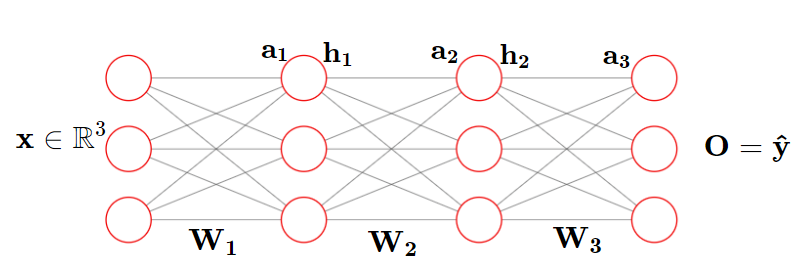
a^l=W^lh^{l-1}+b^l
h^l=\Phi(a^l)
We have only two operations in the entire neural network: Multiply and Add
1. Matrix Multiplication
2. Element-wise addition and (non-linear) transformation
What if some functions or operators that I am looking for is not there in the PyTorch?
Implement forward and backward pass in the autograd.Functions and check the implementation with autograd.gradcheck (finite diff computation).
If you are sure that your function can not be create using composite function (combination of functions and operators that exist already), then you have to write your own.
torch.nn.Module
Developing Deep Learning Models using
Pytorch
Arun Prakash A
DL Course Instructor
BS, IIT Madras, POD
# parameter initialization
W1 = torch.randn(size=(10,2), requires_grad=True)
b1 = torch.randn(size=(10,1), requires_grad=True)
....
for i in range(epochs):
    #forward prop
  for i in range(len(X)):
    a1 = torch.matmul(W1,X[(i,),:].T)+b1
    h1 = torch.sigmoid(a1)
    a2 = torch.matmul(W2,h1)+b2
    h2 = torch.sigmoid(a2)
    a3 = torch.matmul(W3,h2)+b3
    y_hat = torch.sigmoid(a3)
    #Loss function
    L = (1/1000)*torch.pow((y_hat-y[i]),2)
    acc_loss += L.detach().item()

    # backprop
    L.backward()

	# Optimizer
  with torch.no_grad():
    W1  -= eta*W1.grad
    b1  -= eta*b1.grad
    ...

  W1.grad.zero_()
  b1.grad.zero_()
 ...
We can see five sections of code here,
1.Parameter Initialization
2. Forward Propagation
3.Loss function
4. Backprop
5.Optimization
Which section(s) can be automated?
Given a few info, you can construct the rest..?
Module in pytorch means layers in other frameworks (of course, we are also accustomed to the latter "layers" :-))
The core steps involved in the training loop when we use the tensors alone are as follows
#Parameter initialization
w =
b =
for i in range(epochs):

  #Forward prop
  .
  .
  use suitable loss function
  # compute gradients

  loss.backward()

  # context manager
  with torch.no_grad():
    #update all parameters
    .
    use suitable optimizer
    .
    .

  .zero_grad
-
What if we have a really big architecture with millions/billions of parameters?
-
What if we want to use different loss functions and optimizers for tracing/profiling?
-
Moving to
eval()or inference mode?
x = torch.tensor()
W = torch.tensor(requires_grad=True)
b = torch.tensor(reequires_grad=True)
y = torch.matmul(W,x)+b
Layers
x
W
b
@
+
Given the input dim and output dim we can infer the size of parameters
Since this is one of the most frequently used operations in NN, we can wrap it around in a single block (layer) (making an abstraction out of it)
y
Call it a Linear Layer
This is called Modularization
Linear
Convolution
Embedding
RNN
class LinearLayer(nn.Module):

  def __init__(self,in_features,out_features):
    super(LinearLayer,self).__init__()
    self.in_features = in_features
    self.out_features = out_features
    self.w = nn.Parameter(torch.randn(in_features, out_features))
    self.b = nn.Parameter(torch.randn(out_features))

  def forward(self,x):
    out = torch.matmul(x,self.w)+self.b
Let's create a simple linear neuron with the parameters \(w,b\)
The constructor takes in arguments that are required to initialize the network (in this case, input dim and output dim)
All the variables in the base modules are initialized via a super() call.
The parameters W, b are added to the _parameter dict
The forward method has to be defined, the backprop is automated!
class Module:

  # Annotations
  training: bool
  _parameters: Dict[str, Optional[Parameter]]
  _buffers: Dict[str, Optional[Tensor]]
  _non_persistent_buffers_set: Set[str]
  _backward_pre_hooks: Dict[int, Callable]
  _backward_hooks: Dict[int, Callable]
  _is_full_backward_hook: Optional[bool]
  _forward_hooks: Dict[int, Callable]
  _forward_hooks_with_kwargs: Dict[int, bool]
  _forward_pre_hooks: Dict[int, Callable]
  _forward_pre_hooks_with_kwargs: Dict[int, bool]
  _state_dict_hooks: Dict[int, Callable]
  _load_state_dict_pre_hooks: Dict[int, Callable]
  _state_dict_pre_hooks: Dict[int, Callable]
  _load_state_dict_post_hooks: Dict[int, Callable]
  _modules: Dict[str, Optional['Module']]
Base class
Observe that almost all the state variables (including parameters) are stored in dictionaries (make sense)
class Module:

  def __init__(self):

    torch._C._log_api_usage_once("python.nn_module")

    super().__setattr__('training', True)
    super().__setattr__('_parameters', OrderedDict())
    super().__setattr__('_buffers', OrderedDict())
    super().__setattr__('_non_persistent_buffers_set', set())
    super().__setattr__('_backward_pre_hooks', OrderedDict())
    super().__setattr__('_backward_hooks', OrderedDict())
    super().__setattr__('_is_full_backward_hook', None)
    super().__setattr__('_forward_hooks', OrderedDict())
    super().__setattr__('_forward_hooks_with_kwargs', OrderedDict())
    super().__setattr__('_forward_pre_hooks', OrderedDict())
    super().__setattr__('_forward_pre_hooks_with_kwargs', OrderedDict())
    super().__setattr__('_state_dict_hooks', OrderedDict())
    super().__setattr__('_state_dict_pre_hooks', OrderedDict())
    super().__setattr__('_load_state_dict_pre_hooks', OrderedDict())
    super().__setattr__('_load_state_dict_post_hooks', OrderedDict())
    super().__setattr__('_modules', OrderedDict())
Base class
Using ordered dict is a right choice (why does order matter here?)
CNN for Image classification
- TorchData
Developing Deep Learning Models using
Pytorch
Arun Prakash A
DL Course Instructor
BS, IIT Madras, POD
| 1 |
|---|
| 2 |
| 3 |
| 4 |
| 5 |
| 6 |
| 7 |
| 8 |
| 9 |
| 10 |
| 11 |
| 12 |
| 13 |
| 14 |
| 15 |
| 16 |
| 17 |
| 18 |
N samples
in a storage
X
What we have so far
torch.tensor
Torch.nn.module
(Linear, Conv2D,
RNN)
torch.optim

.Step
We could build any deep learning model with these modules
torch.nn.Parameter
torch.autograd
\theta,\nabla \theta
\theta-\nabla \theta
How do we feed in the data to the mode for training?
We can slice the batch and iterate, not a big deal

| 1 |
|---|
| 2 |
| 3 |
| 4 |
| 5 |
| 6 |
| 7 |
| 8 |
| 9 |
| 10 |
| 11 |
| 12 |
| 13 |
| 14 |
| 15 |
| 16 |
| 17 |
| 18 |
N samples
in a storage
| 1 |
|---|
| 10 |
| 5 |
| 4 |
| 3 |
| 6 |
| 17 |
| 8 |
| 9 |
| 2 |
| 11 |
| 16 |
| 13 |
| 14 |
| 15 |
| 12 |
| 7 |
| 18 |
Shuffled indices
X
X

Model Under
training
We can't fetch the next set of batches simultaneously when the model is being trained
Fetch
(Model waits until samples are fetched)
This is due to pythons GIL
Then, what is the purpose of TorchData?
# Load entire dataset
X, y = torch.load('some_training_set_with_labels.pt')

# Train model
for epoch in range(max_epochs):
    for i in range(n_batches):
        # Local batches and labels
        local_X, local_y = X[i*n_batches:(i+1)*n_batches,], y[i*n_batches:(i+1)*n_batches,]

        # Your model
        [...]
Could you think of some drawbacks of loading data in this way?
Especially, putting the model and data loading into the same loop
Overloads Memory by (unnecessarily) loading all sample
The model waits for some time to get it samples (due to pythons GIL)
Data processing is a complex task (especially for NLP)
It involves tasks like Pre-processing (transforming), collating into batches, distributing across machines...
Having a separate module(functions) to do them makes code clean and neat.
TorchData module does that exactly with the help of dataset (datapipe in beta stage) and dataloader classes
Moreover, we do not want to transform all samples in the dataset all at once (otherwise, consumes a lot of memory)
Dataset: Map Style
We need to inherit the abstract class from torch.utils.data.Dataset and must implement a __getitem__ and __len__ method that returns a single sample from the dataset
class Dataset():

  def __getitem__(self, index) :
        raise NotImplementedError

  def __add__(self, other) :
      return ConcatDataset([self, other])
class MyDataset(Dataset):
def __init__(self,path_to_dataset):
self.path = 'path_to_dataset'
def __getitem__(self, index) :
# Load data using appropriate library
.
#Preprocess - transform
#
return a_single_sample, label
def __add__(self, other) :
# implement how to concatenate
# else default will be considered
return ConcatDataset([self, other])We call it map because it maps an indices/keys (idx) to samples. This is suitable if you have an off-line (stored in disk) dataset. That is, all samples are available at once
What if my data is of online (streaming)? possibly coming from multiple streams
Dataset: iterable- Style
From doc:
" This type of datasets is particularly suitable for cases where random reads are expensive or even improbable, and where the batch size depends on the fetched data."
Natural Language Processing
" This course contents are well organised"
Recurrent Neural Network
[{Label:'Positive', Score:0.997}]" The course contents are well organized"
Recurrent Neural Network
[{Label:'Positive', Score:0.997}]Tokenize
[The, course,contents,are,well,organized]
Numericalize
[{The:10, course:18,contents:14,are:100,well:9,organized:6982}]Embedding
[random initialization, word2vec, glove, fasttext..]
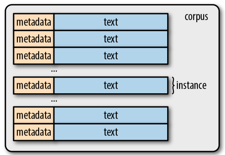
Corpora - Token
Corpus: collections of raw text (in ASCII or UTF-8)
A sequence of characters (bytes)
Group them into contiguous units called tokens (ex, words, numeric seq, punctuations)
Tokenization
A process that breaks text into tokens
It is a highly complicated process, task specific, arbitrary but extremely important step
Types
Unique tokens in a corpus
A set of all types in a corpus is its vocubulary (A set of all unique tokens in the text is its vocabulary or lexicon)
Words are of two types: content words and stop words (articles, prepositions..)
Corpus: {"The mouse eat the cheese.",
"The mouse is really good to use!"}
\(\mathcal{V}:\) {the, mouse,eat, cheese, is, really good, to ,use,!}
N-Grams
n-consecutive token sequences in a text (not in a vocubulary)
Unigram: {"the", "mouse", "eat", ..}
Corpus: {"The mouse eat the cheese.",
"The mouse is really good to use!"}
Corpus: {"The mouse eat the cheese.",
"The mouse is really good to use!"}
Bigram: {"the mouse", "mouse eat", "eat the", ..}
Trigram: {"the mouse eat", "mouse eat the", "eat the cheese", ..}
Character level tokens are sometimes helpful. Those tokens are subwords in a word. Say, "-ol" in methonol, ethanol
lemmas
lemmas are root forms of words
be : is,was,were
fly : flow, flowed, flying..
Often used in traditional nlp to reduce the dimension of a vector representation.
It can also be cast as a learning problem (instead of handcrafting rules).
Torchtext
All texts (samples) from a corpus
Tokenize
(basic, subword, bpe)
Build vocabulary
(tokens to indices)
from torchtext.datasets import IMDB
train_iter = IMDB(root='./data',split='train')
all_samples = list(train_iter)
from torchtext.data.utils import get_tokenizer
tokenizer = get_tokenizer(tokenizer="basic_english",language='en')
counter=Counter()
for (label,sent) in all_samples: # iterate over all samples
  counter. Update(tokenizer(sent))
v1 = vocab(counter,min_freq=1,specials=[unk_token]) #build vocabulary
v1.set_default_index(default_index)
Task: Take a sentence and return a sequence of tokens as defined by tokenizer
Task: Dictionary of tokens {token-1: frequency, token-2: frequency, ..., token_n : frequency}
Note: We count the frequency of a token, so that we can decide whether the token be a part of vocabulary based on its freq value
Now, the vocab function assigns an integer (index) to each token
We can make use of the index to create a vector representation of words or sentences in multiple ways, for example
| I | am | proud | of | you | made | me |
|---|---|---|---|---|---|---|
| 0 | 1 | 2 | 3 | 4 | 5 | 6 |
I am
Sentence to vector
[0,1]
you made me proud
[0,1]
Word to vector (one-hot-encoding)
I
[1,0,0,0,0,0,0]
made
[0,0,0,0,0,1,0]
Say, |V| = 7 as follows
Embedding Layer
Given the index \(i\) for a token, get me a vector representation \(x_i\) of size \(k\)
We need a vector representation for each token. Initially all the vectors are purely random (as we initialize the parameters)
|V| \times k
The embedding layer is just a HUGE trainable look-up table !
i
x_i=[0.1,-0.1,0.8,\cdots,0.35]_{1 \times k}
If we have \(|V|\) of size 1 million, and \(k=50\), then we need to learn 50 million parameters
Challenges:
1. Vocabulary changes from dataset to dataset
2. Word embeddings may not contain embedding for all words in your vocabulary
3. Therefore, we need to use embedding layer and initialize the weights for words, not in the vocabulary of pre-trained word-embeddings, randomly
Build Transformers from scratch
(using pytorch nn.module)
Arun Prakash A
IIT Madras
Encoder
def scaled_dot_product_attention(Q, K, V):
   dim_k = K.size(-1)
   scores = torch.bmm(Q, K.transpose(1, 2)) / sqrt(dim_k)
   weights = F.softmax(scores, dim=-1)
   return torch.bmm(weights, V)
Scaled Dot Product
Q
K
V
\text{MatMul:} \ QK^T
\text{Scale}:\frac{1}{\sqrt{d_k}}
\text{Softmax}
\text{MatMul}
Scaled Dot Product
Head
Q
K
V
W_Q
W_K
W_V
H=\{h_1,h_2,\cdots,h_T\}
Attention Head
class AttentionHead(nn.Module):
   def __init__(self, embed_dim=512, head_dim=64):
     super().__init__()
     self.q = nn.Linear(embed_dim, head_dim)
     self.k = nn.Linear(embed_dim, head_dim)
     self.v = nn.Linear(embed_dim, head_dim)
   def forward(self, hidden_state):
     attn_outputs = scaled_dot_product_attention(
     				self.q(hidden_state),
       				self.k(hidden_state),
       				self.v(hidden_state))
     return attn_outputs
DirectChat - Lmarena
DirectChat - arena.ai4bharat.org
Concatenate (:\(T \times 512\))
Linear
W_Q^8
W_K^8
W_V^8
Scaled Dot Product
Attention
W_Q^2
W_K^2
W_V^2
Scaled Dot Product
Attention
Scaled Dot Product
Attention
h_j
h_j
h_j
W_Q^1
W_K^1
W_V^1
Multi-Head Attention
class MultiHeadAttention(nn.Module):
   def __init__(self, embed_dim=512,num_head=8):
     super().__init__()
     head_dim = embed_dim//num_heads # 512/8 = 64

     # create 8 heads as pytorch module using ModuleList
     self.heads = nn.ModuleList(
     [AttentionHead(embed_dim, head_dim) for _ in range(num_heads)]
     )
     self.output_linear = nn.Linear(embed_dim, embed_dim)

    def forward(self, hidden_state):
     x = torch.cat([h(hidden_state) for h in self.heads], dim=-1)
     x = self.output_linear(x)
     return x
I
enjoyed
the
movie
transformers
Encoder Layer
Feed Forward Network
Multi-Head Attention
class FeedForward(nn.Module):

   def __init__(self):
     super().__init__()
     self.linear_1 = nn.Linear(512, 2048)
     self.linear_2 = nn.Linear(2048, 512)
     self.gelu = nn.GELU()
     self.dropout = nn.Dropout(0.5)

   def forward(self, x):
     x = self.linear_1(x)
     x = self.gelu(x)
     x = self.linear_2(x)
     x = self.dropout(x)
     return x
Encoder
Feed Forward Network
Multi-Head Attention
Add & Layer Norm
Add & Layer Norm
class TransformerEncoderLayer(nn.Module):

 def __init__(self,config):
   super().__init__()
   self.layer_norm_1 = nn.LayerNorm(config.hidden_size)
   self.layer_norm_2 = nn.LayerNorm(config.hidden_size)
   self.attention = MultiHeadAttention(config)
   self.feed_forward = FeedForward(config)

 def forward(self, x):
   # Apply layer normalization and then copy input into query, key, value
   hidden_state = self.layer_norm_1(x)
   # Apply attention with a skip connection
   x = x + self.attention(hidden_state)
   # Apply feed-forward layer with a skip connection
   x = x + self.feed_forward(self.layer_norm_2(x))
   return x
BERT
Preparing Data
All texts (samples) from a corpus
Sentence Tokenizer, Word Tokenizer
(basic, subword, bpe)
Build vocabulary
(tokens to indices)
Step-1
Get input ids for each token in batch of (N)samples
Randomly replace tokens with <mask> token
Pad tokens for batching samples in data loader
Ensure all samples are of same length by padding <pad> token ids
dtype: list
dtype: list
dtype: tensor
Step-2
Pytorch
By Arun Prakash
Pytorch
A walkthrough over Pytorch framework to develop dl models using both low level and high-level APIs


